批梯度下降随机梯度下降_什么是梯度下降

最新推荐文章于 2021-05-26 19:04:49 发布

杨_明

最新推荐文章于 2021-05-26 19:04:49 发布

阅读量173

点赞数

文章标签：深度学习 python 神经网络机器学习人工智能

原文链接：https://medium.com/analytics-vidhya/what-is-gradient-descent-e59d981d5cdb

版权

批梯度下降随机梯度下降

总览(Overview)

This tutorial is on the basics of gradient descent. It is also a continuation of the Intro to Machine Learning post, “What is Machine Learning?”, which can be found here.

本教程基于梯度下降的基础。这也是“机器学习入门”帖子“什么是机器学习？”的续篇，可以在这里找到。

那么什么是梯度下降？ (So what is gradient descent?)

Gradient descent is a method of finding the optimal weights for a model. We use the gradient descent algorithm to find the best machine learning model, with the lowest error and highest accuracy. A common explanation of gradient descent is the idea of standing on an uneven baseball field, blindfolded, and you want to find the lowest point of the field. Naturally, you will use your feet to inch your way to the lowest point on the field. Looking for any downward slope. Conceptually, this is what we are doing to minimize our error and find our best performing machine learning model.

梯度下降是一种找到模型最佳权重的方法。我们使用梯度下降算法来找到最佳的机器学习模型，具有最低的误差和最高的准确性。梯度下降的一个常见解释是站在不平坦的棒球场上，蒙住双眼，而您想找到该场的最低点。自然，您将用脚踩到底，直至到达最低点。寻找任何向下的坡度。从概念上讲，这是我们要做的，以最大程度地减少错误并找到性能最佳的机器学习模型。

这与第一个教程中的y = mx + b方程有什么关系？ (How does this relate to our y = mx + b equation in the first tutorial?)

We can calculate derivatives, our error, and update our weights (a.k.a. m and b).

我们可以计算导数，我们的误差并更新权重(即m和b )。

例 (Example)

Let’s get started. The only two libraries we will be using are numpy and matplotlib. Numpy is a great library for mathematical computations, whereas matplotlib is used for visualizations and graphing.

让我们开始吧。我们将使用的仅有的两个库是numpy和matplotlib。 Numpy是一个很好的数学计算库，而matplotlib用于可视化和图形绘制。

导入我们将要使用的库 (Importing libraries we will be using)

# Numpy is a powerful library in Python to do mathemetical computations
import numpy as np

# Importing matplotlib for visualizations
from matplotlib import pyplot as plt

我们可以创建一些符合以下等式的数据： `y = 4x + 2`其中`m` = 4， `b` = 2 (We can create some data that will follow this equation: `y = 4x + 2` where `m` = 4, `b` = 2)

Since we know the ground truth, we can create some data that follows this equation. We can also compare our weights calculated using gradient descent to the ground truth, where m = 4 and b = 2.

由于我们知道基本事实，因此我们可以创建一些遵循此等式的数据。我们还可以将使用梯度下降法计算的权重与地面真实情况进行比较，其中m = 4，b = 2。

X = np.array([1, 2, 3, 4, 5, 6, 7, 8, 9, 10])
y = np.array([6, 10, 14, 18, 22, 26, 30, 34, 38, 42])

plt.plot(X, y)
plt.title('Made up data following the equation y = 4x + 2')
plt.ylabel('y')
plt.xlabel('X')
plt.show()

Now let’s create a Gradient Descent function in Python

现在让我们在Python中创建一个Gradient Descent函数

def gradient_descent(x, y, learning_rate, steps):
    # Randomly initialize m and b. Here we set them to 0.
    m = b = 0
    
    # N is just the number of observations
    N = len(x)
    
    # Creating an empty list to plot how the error changes
    # over time later on with matplotlib.
    error_history = list()
    
    # Loop through the number of iterations specified to get closer to the optimal model
    for i in range(steps):
        # Since y = mx + b, we predict y is going to be m * x + b
        y_predicted = (m * x) + b
        
        # We calculate the error for each model we try, attempting to get the least amount of error possible
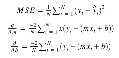
        # In this case we calculate the mean squared error (MSE)
        error = (1 / N) * sum([value ** 2 for value in (y - y_predicted)])
        # Append to the error history, so we can visualize later
        error_history.append(error)
        
        # Calculate the partial derivatives for m and b
        dm = (-2 / N) * sum(x * (y - y_predicted))
        db = (-2 / N) * sum((y - y_predicted))
        
        # Update m and b based on the partial derivatives and the specified learning rate
        m = m - learning_rate * dm
        b = b - learning_rate * db
        
        # Print the step number, error, and weights
        print(f"Step {i + 1} \n Error = {error} \n m = {m} \n b = {b} \n")
        
    return m, b, error_history

让我们分解一下这个功能 (Let’s break this function down)

First we set m and b equal to 0. This is to randomly intitialize these variables, you can set them to whatever value you want.
首先，我们将m和b设置为0。这是为了随机初始化这些变量，您可以将它们设置为所需的任何值。

2. Then we find how many data points we have and put that as variable N

2.然后我们找到多少个数据点并将其作为变量N

3. We create an empty array to save the history of the error (remember, error is the difference between what we predicted and the actual value)

3.我们创建一个空数组来保存错误的历史记录(请记住，错误是我们预测的值与实际值之间的差)

4. Finally, we create the gradient descent loop:

4.最后，我们创建梯度下降循环：

First, within the loop, we calculate our predicted point which is y in mx + b. So, we end up with y_predicted = mx + b
首先，在循环中，我们计算出预测点，即mx + b中的y。因此，我们最终得到y_predicted = mx + b
We calculate the error for each point we predicted. In this case we use mean squared error (MSE). This is calculated by finding the error, then squaring it, and then taking the average of all of the squared errors.
我们为预测的每个点计算误差。在这种情况下，我们使用均方误差(MSE)。这是通过找到误差，然后对它进行平方，然后取所有平方误差的平均值来计算的。
Then we add the MSE to the history array to visualize later.
然后，我们将MSE添加到历史记录数组中，以便以后进行可视化。
Now, we do something very important and fundamental for the gradient descent algorithm — we calculate the partial derivatives for our weights. A partial derivative just holds the other variables constant while you figure out how the variable you are observing behaved during the process.
现在，我们对梯度下降算法进行了非常重要且基本的工作-我们计算了权重的偏导数。当您弄清楚所观察的变量在此过程中的行为时，偏导数仅使其他变量保持不变。
Then we update our weights m and b according to the partial derivatives and the learning rate we specified. (Learning rate is how large of a step you are taking)
然后，我们根据偏导数和指定的学习率更新权重m和b 。 (学习率是您迈出的第一步)
Then finally we print out the values and return the variables.
最后，我们打印出值并返回变量。

Formulas:

公式：

We can specify how many “steps” we want the gradient descent algorithm to run. Essentially, how many steps you are allowed to make on that baseball field while blindfolded.

我们可以指定要运行梯度下降算法的“步数”。本质上，被蒙住眼睛时允许您在那个棒球场上执行多少步骤。

steps = 5

We can also specify the “learning rate”, which will tell us how big those steps are. Conceptually, think about how big of a step you are allowed to take, each time you take one on the baseball field. Too big of a step could cause you to over-shoot the lowest point of the field. However, too small of a step will make it take longer for you to find the lowest point. This variable becomes more widely talked about in deep learning. For now we will set it to 0.01.

我们还可以指定“学习率”，这将告诉我们这些步骤有多大。从概念上讲，考虑一下您每次在棒球场上迈出的步伐有多大。太大的步骤可能会导致您超出该字段的最低点。但是，步骤太小会导致您花费更长的时间找到最低点。在深度学习中，这个变量变得更为广泛地讨论。现在我们将其设置为0.01。

learning_rate = 0.01

Now let’s run our made-up data through gradient descent and see what m and b values pop out.

现在，让我们通过梯度下降来运行人造数据，看看弹出的m和b值是多少。

m, b, error_history = gradient_descent(X, y, learning_rate, steps)

[Output]

[输出]

Step 1

第1步

Error = 708.0, m = 3.3000000000000003, b = 0.48

误差= 708.0，m = 3.3000000000000003，b = 0.48

…

…

Step 5

第5步

Error = 0.40731798550902065, m = 4.194540273, b = 0.6321866478

误差= 0.40731798550902065，m = 4.194540273，b = 0.6321866478

Notice, the error continues to decrease and m approaches 4 while b approaches 2. If we increase the number of steps the algorithm is allowed to take, it will get even closer to the real values.

请注意，误差继续减小， m接近4，而b接近2。如果我们增加允许算法执行的步骤数，则它将更加接近真实值。

steps = 10
m, b, error_history = gradient_descent(X, y, learning_rate, steps)

[Output]

[输出]

Step 1

第1步

Error = 708.0, m = 3.3, b = 0.48

误差= 708.0，m = 3.3，b = 0.48

…

…

Step 10

第10步

Error = 0.3875, m = 4.19234, b = 0.66093

误差= 0.3875，m = 4.19234，b = 0.66093

You can see with more steps, we get closer to the real m and b values of 4 and 2!

您可以看到更多的步骤，我们更接近4和2的实际m和b值！

让我们看一下错误在每个步骤之后如何变化 (Let’s take a look at how the error changed after each step)

plt.plot(range(steps), error_history)
plt.title('Error over time')
plt.ylabel('Error')
plt.xlabel('Number of Steps')
plt.show()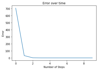

As we can see, it sharply declines. Then it slowly gets lower. You will see this type of plot often when training deep learning or other machine learning models.

如我们所见，它急剧下降。然后它慢慢降低。在训练深度学习或其他机器学习模型时，您会经常看到这种类型的图。

现在，让我们看一下梯度下降算法得出的线，并用实际线绘制。 (Now let’s look at the line the gradient descent algorithm came up with, plotted with the actual line.)

y_predicted = (m * X) + b

plt.plot(X, y)
plt.plot(X, y_predicted)
plt.title('Estimation Using Gradient Descent')
plt.ylabel('y')
plt.xlabel('X')
plt.legend(["Actual", "Estimated using Gradient Descent"])
plt.show()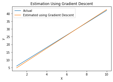

We can see the gradient descent algorithm did a pretty good job! If we allowed gradient descent to run even longer, it would be able to lineup even closer to the actual function in this plot.

我们可以看到梯度下降算法做得很好！如果我们允许梯度下降运行更长的时间，它将能够更接近该图中的实际功能。

概要 (Summary)

To conclude, gradient descent is an algorithm to optimize a machine learning model. It attempts to find the best weights for the model, in order to approximate a function found in data. Over time, the errors will (hopefully) decrease and accuracy will increase. In order to do this, the gradient descent algorithm calculates the partial derivatives of the weights. These partial derivatives tell the algorithm in which direction to update the weights. While the learning rate tells us how large of a step the weights are allowed to take, in the direction given by the partial derivatives.

总而言之，梯度下降是一种优化机器学习模型的算法。它试图找到模型的最佳权重，以便近似数据中找到的函数。随着时间的流逝，错误将(希望)减少，准确性将会提高。为此，梯度下降算法计算权重的偏导数。这些偏导数告诉算法更新权重的方向。虽然学习率告诉我们，在偏导数给出的方向上，权重允许执行多大的步长。