使用机器学习模型预测贷款资格

介绍(Introduction)

Loans are the core business of banks. The main profit comes directly from the loan’s interest. The loan companies grant a loan after an intensive process of verification and validation. However, they still don’t have assurance if the applicant is able to repay the loan with no difficulties.

贷款是银行的核心业务。 主要利润直接来自贷款利息。 贷款公司经过大量的验证和确认过程后才发放贷款。 但是，他们仍然不确定申请人是否能够无困难地偿还贷款。

In this tutorial, we’ll build a predictive model to predict if an applicant is able to repay the lending company or not. We will prepare the data using Jupyter Notebook and use various models to predict the target variable.

在本教程中，我们将建立一个预测模型，以预测申请人是否能够偿还贷款公司。 我们将使用Jupyter Notebook准备数据，并使用各种模型来预测目标变量。

目录 (Table of Contents)

1. Getting the system ready and loading the data
   准备系统并加载数据
2. Understanding the data
   了解数据

3. Exploratory Data Analysis (EDA)

   探索性数据分析(EDA)

   i. Univariate Analysis

   一世。 单变量分析

   ii. Bivariate Analysis

   ii。 双变量分析

4. Missing value and outlier treatment
   价值缺失和异常值处理
5. Evaluation Metrics for classification problems
   分类问题的评估指标
6. Model Building: Part 1
   模型制作：第1部分
7. Logistic Regression using stratified k-folds cross-validation
   使用分层k折交叉验证的Logistic回归
8. Feature Engineering
   特征工程

9. Model Building: Part 2

   模型制作：第2部分

   i. Logistic Regression

   一世。 逻辑回归

   ii. Decision Tree

   ii。 决策树

   iii. Random Forest

   iii。 随机森林

   iv. XGBoost

   iv。 XGBoost

准备系统并加载数据 (Getting the system ready and loading the data)

We will be using Python for this course along with the below-listed libraries.

本课程将使用Python和下面列出的库。

Specifications

技术指标

• Python
  Python
• pandas
  大熊猫
• seaborn
  海生的
• sklearn
  斯克莱恩

import pandas as pd
import numpy as np
import seaborn as sns
import matplotlib.pyplot as plt
%matplotlib inline
import warnings
warnings.filterwarnings(“ignore”)

数据 (Data)

For this problem, we have three CSV files: train, test, and sample submission.

对于此问题，我们有三个CSV文件：训练，测试和样品提交。

• Train file will be used for training the model, i.e. our model will learn from this file. It contains all the independent variables and the target variable.

  训练文件将用于训练模型，即我们的模型将从该文件中学习。 它包含所有自变量和目标变量。

• Test file contains all the independent variables, but not the target variable. We will apply the model to predict the target variable for the test data.

  测试文件包含所有自变量，但不包含目标变量。 我们将应用该模型预测测试数据的目标变量。

• Sample submission file contains the format in which we have to submit out predictions

  样本提交文件包含我们必须提交预测的格式

读取数据(Reading data)

train = pd.read_csv(‘Dataset/train.csv’)
train.head()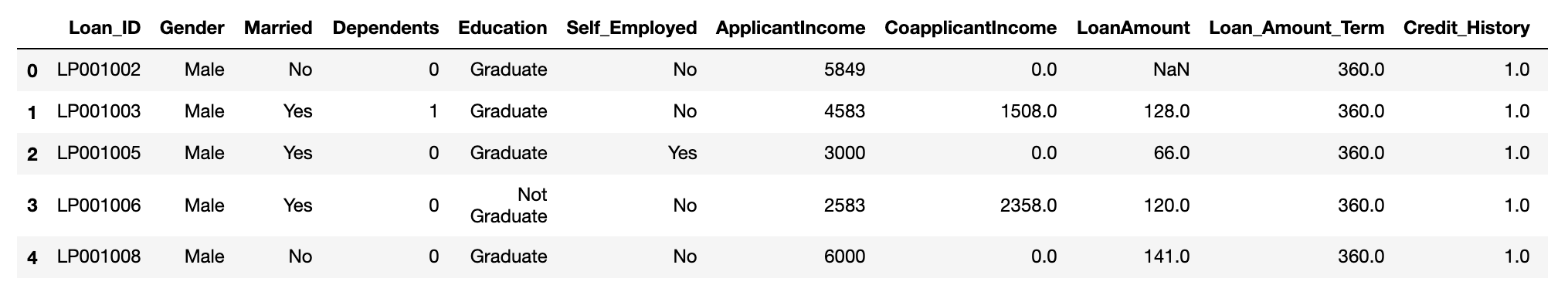

test = pd.read_csv(‘Dataset/test.csv’)
test.head()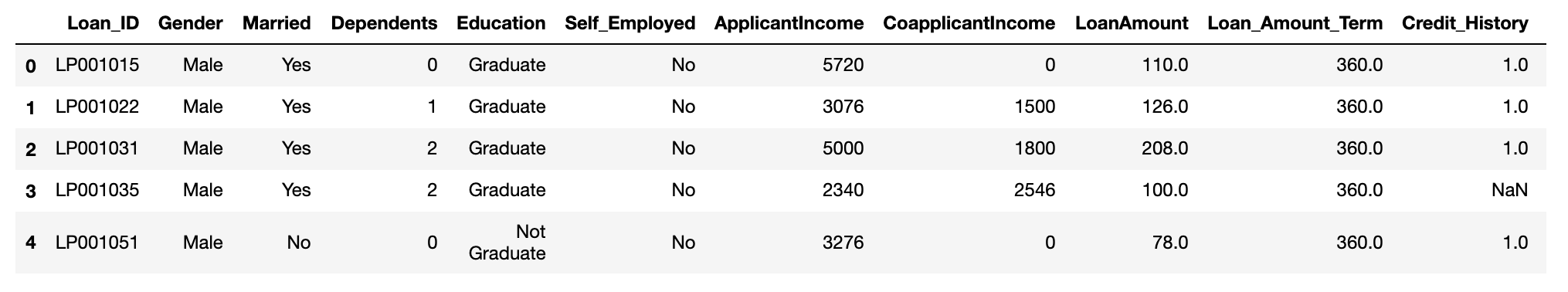

Let’s make a copy of the train and test data so that even if we have to make any changes in these datasets we would not lose the original datasets.

让我们复制训练和测试数据，以便即使我们必须对这些数据集进行任何更改，也不会丢失原始数据集。

train_original=train.copy()
test_original=test.copy()

了解数据 (Understanding the data)

train.columnsIndex(['Loan_ID', 'Gender', 'Married', 'Dependents', 'Education',
       'Self_Employed', 'ApplicantIncome', 'CoapplicantIncome', 'LoanAmount',
       'Loan_Amount_Term', 'Credit_History', 'Property_Area', 'Loan_Status'],
      dtype='object')

We have 12 independent variables and 1 target variable, i.e. Loan_Status in the training dataset.

我们有12个自变量和1个目标变量，即训练数据集中的Loan_Status。

test.columnsIndex(['Loan_ID', 'Gender', 'Married', 'Dependents', 'Education',
       'Self_Employed', 'ApplicantIncome', 'CoapplicantIncome', 'LoanAmount',
       'Loan_Amount_Term', 'Credit_History', 'Property_Area'],
      dtype='object')

We have similar features in the test dataset as the training dataset except for the Loan_Status. We will predict the Loan_Status using the model built using the train data.

除了Loan_Status外，我们在测试数据集中与训练数据集具有相似的功能。 我们将使用火车数据构建的模型预测Loan_Status。

train.dtypesLoan_ID               object
Gender                object
Married               object
Dependents            object
Education             object
Self_Employed         object
ApplicantIncome        int64
CoapplicantIncome    float64
LoanAmount           float64
Loan_Amount_Term     float64
Credit_History       float64
Property_Area         object
Loan_Status           object
dtype: object

We can see there are three formats of data types:

我们可以看到三种类型的数据类型：

• object: Object format means variables are categorical. Categorical variables in our dataset are Loan_ID, Gender, Married, Dependents, Education, Self_Employed, Property_Area, Loan_Status.
  对象：对象格式表示变量是分类的。 我们数据集中的分类变量是Loan_ID，性别，已婚，家属，教育，自雇，Property_Area，Loan_Status。
• int64: It represents the integer variables. ApplicantIncome is of this format.
  int64：表示整数变量。 ApplicantIncome是这种格式。
• float64: It represents the variable that has some decimal values involved. They are also numerical
  float64：它表示包含一些十进制值的变量。 它们也是数值

train.shape(614, 13)

We have 614 rows and 13 columns in the train dataset.

火车数据集中有614行和13列。

test.shape(367, 12)

We have 367 rows and 12 columns in test dataset.

测试数据集中有367行和12列。

train[‘Loan_Status’].value_counts()Y    422
N    192
Name: Loan_Status, dtype: int64

Normalize can be set to True to print proportions instead of number

可以将Normalize设置为True以打印比例而不是数字

train[‘Loan_Status’].value_counts(normalize=True) Y    0.687296
N    0.312704
Name: Loan_Status, dtype: float64train[‘Loan_Status’].value_counts().plot.bar()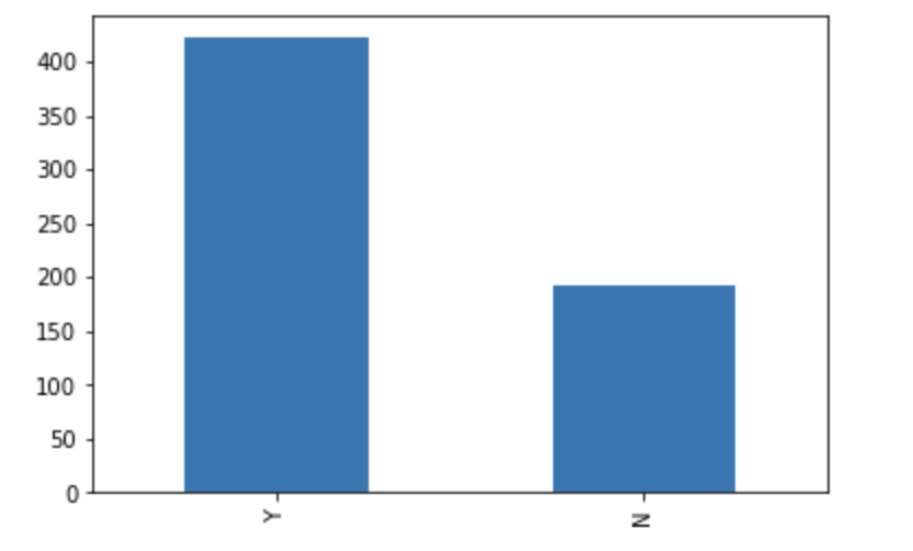

The loan of 422(around 69%) people out of 614 were approved.

批准了614人中的422人(约占69％)的贷款。

Now, let's visualize each variable separately. Different types of variables are Categorical, ordinal, and numerical.

现在，让我们分别可视化每个变量。 不同类型的变量是分类变量，序数变量和数值变量。

• Categorical features: These features have categories (Gender, Married, Self_Employed, Credit_History, Loan_Status)

  分类功能：这些功能具有类别(性别，已婚，自雇，信用历史，贷款状态)

• Ordinal features: Variables in categorical features having some order involved (Dependents, Education, Property_Area)

  顺序特征：分类特征中涉及某些顺序的变量(受抚养人，教育程度，Property_Area)

• Numerical features: These features have numerical values (ApplicantIncome, Co-applicantIncome, LoanAmount, Loan_Amount_Term)

  数值特征：这些特征具有数值(ApplicantIncome，Co-applicantIncome，LoanAmount，Loan_Amount_Term)

自变量(分类) (Independent Variable (Categorical))

train[‘Gender’].value_counts(normalize=True).plot.bar(figsize=(20,10), title=’Gender’)
plt.show()
train[‘Married’].value_counts(normalize=True).plot.bar(title=’Married’)
plt.show()
train[‘Self_Employed’].value_counts(normalize=True).plot.bar(title=’Self_Employed’)
plt.show()
train[‘Credit_History’].value_counts(normalize=True).plot.bar(title=’Credit_History’)
plt.show()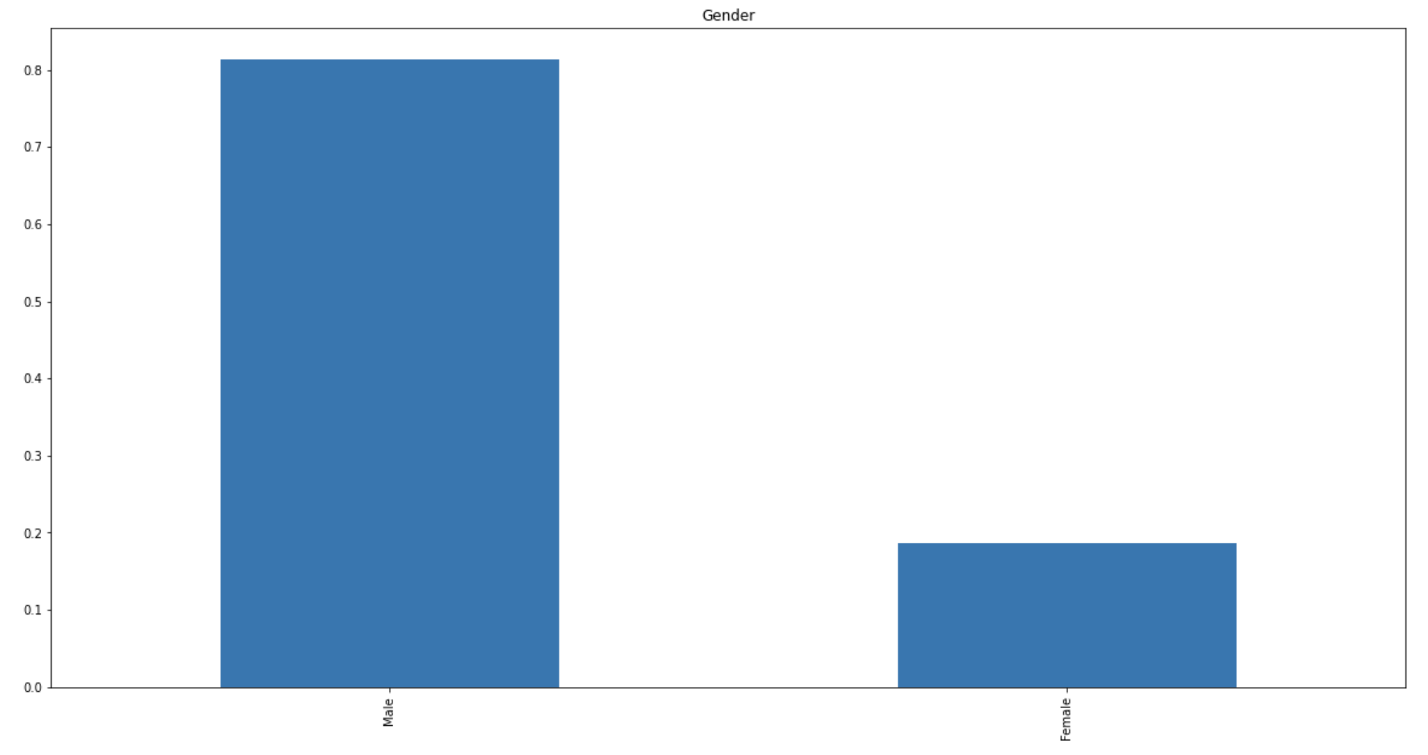

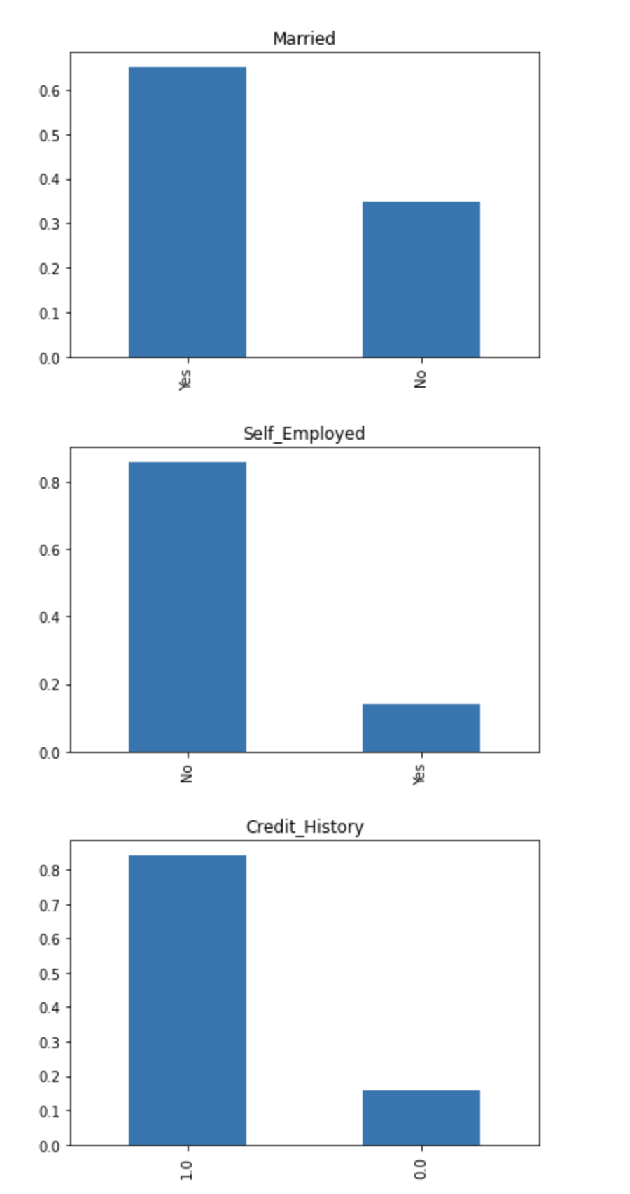
It can be inferred from the above bar plots that:

从上面的条形图中可以推断出：

• 80% of applicants in the dataset are male.
  数据集中80％的申请人是男性。
• Around 65% of the applicants in the dataset are married.
  数据集中约有65％的申请人已婚。
• Around 15% of applicants in the dataset are self-employed.
  数据集中约有15％的申请人是自雇人士。
• Around 85% of applicants have repaid their doubts.
  大约85％的申请人已经解决了他们的疑问。

自变量(序数) (Independent Variable (Ordinal))

train[‘Dependents’].value_counts(normalize=True).plot.bar(figsize=(24,6), title=’Dependents’)
plt.show()
train[‘Education’].value_counts(normalize=True).plot.bar(title=’Education’)
plt.show()
train[‘Property_Area’].value_counts(normalize=True).plot.bar(title=’Property_Area’)
plt.show()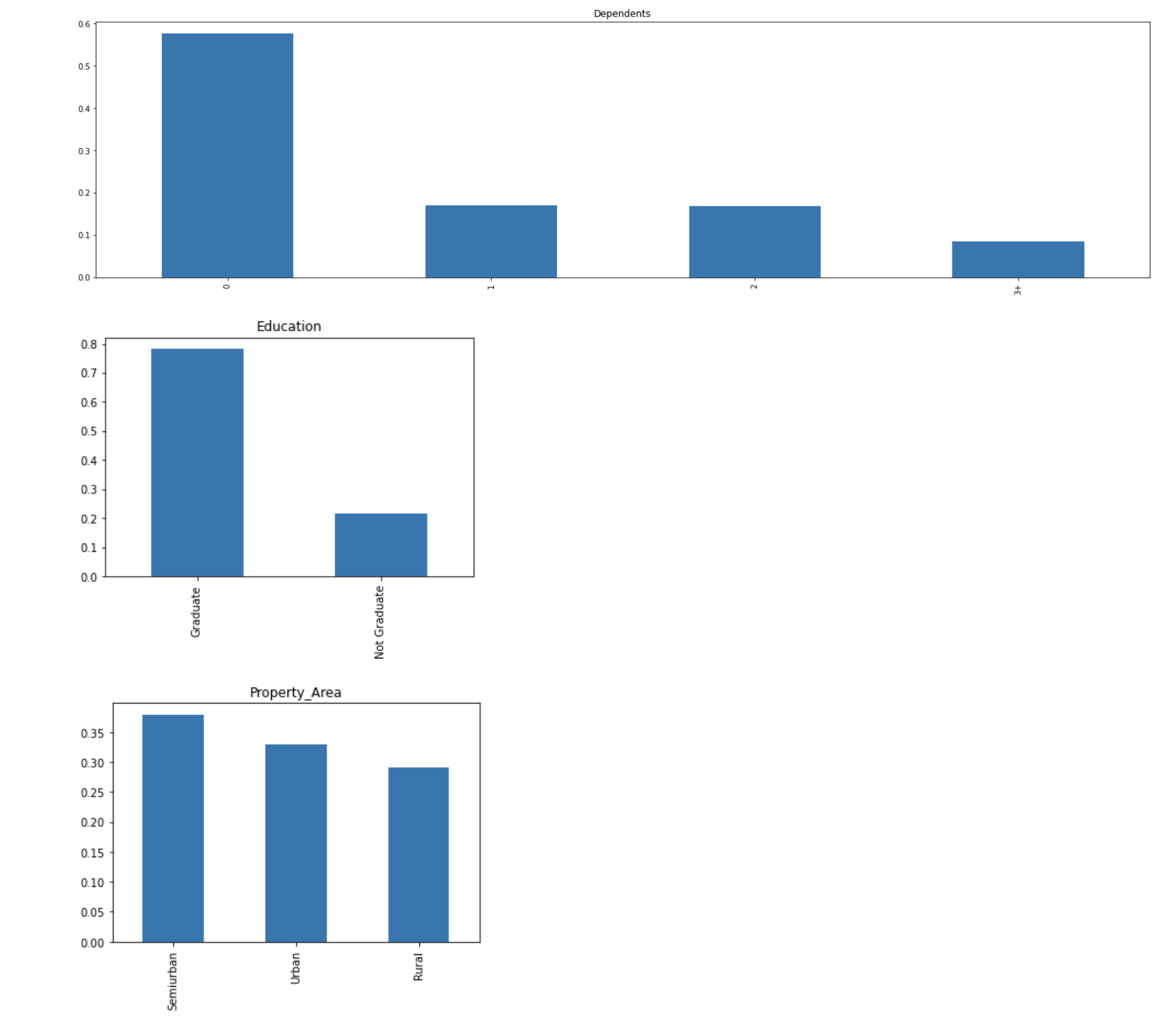

The following inferences can be made from the above bar plots:

从上面的条形图可以得出以下推论：

• Most of the applicants don't have any dependents.
  大多数申请人没有任何受抚养人。
• Around 80% of the applicants are Graduate.
  大约80％的申请者是研究生。
• Most of the applicants are from the Semiurban area.
  大多数申请人来自塞米班地区。

自变量(数值) (Independent Variable (Numerical))

Till now we have seen the categorical and ordinal variables and now let's visualize the numerical variables. Let's look at the distribution of Applicant income first.

到目前为止，我们已经看到了分类变量和序数变量，现在让我们可视化数字变量。 首先让我们看一下申请人收入的分配。

sns.distplot(train[‘ApplicantIncome’])
plt.show()
train[‘ApplicantIncome’].plot.box(figsize=(16,5))
plt.show()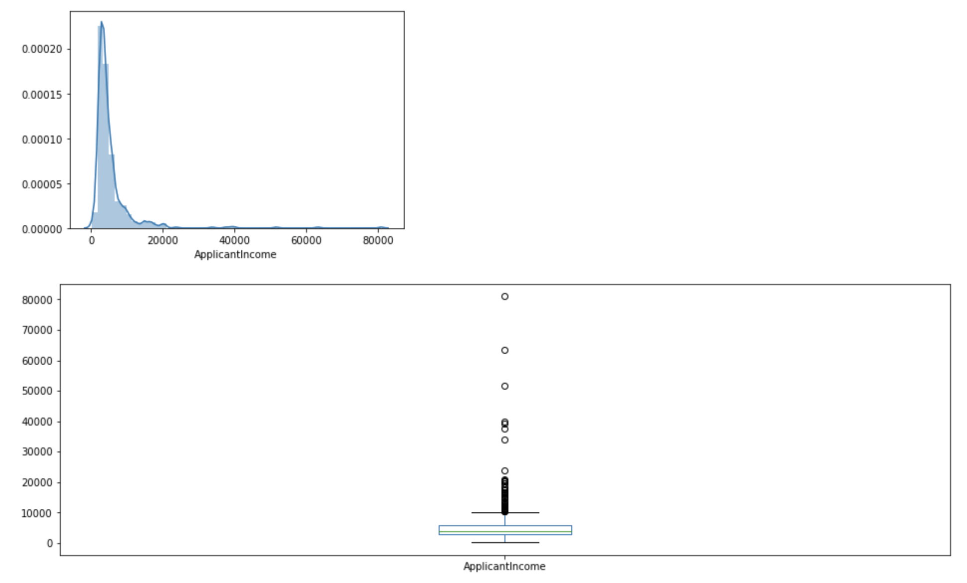

It can be inferred that most of the data in the distribution of applicant income are towards the left which means it is not normally distributed. We will try to make it normal in later sections as algorithms work better if the data is normally distributed.

可以推断，申请人收入分配中的大多数数据都向左，这意味着它不是正态分布。 我们将在后面的章节中尝试使其正常，因为如果数据呈正态分布，则算法会更好地工作。

The boxplot confirms the presence of a lot of outliers/extreme values. This can be attributed to the income disparity in the society. Part of this can be driven by the fact that we are looking at people with different education levels. Let us segregate them by Education.

箱线图确认存在许多异常值/极端值。 这可以归因于社会上的