


机器学习可视化
Yellowbrick is a Python machine learning visualization library. It is essentially built-on Scikit-learn and Matplotlib. Yellowbrick provides informative visualizations to better evaluate machine learning models. It also helps in the process of model selection.
Yellowbrick是Python机器学习可视化库。 它本质上是建立在Scikit-learn和Matplotlib之上的。 Yellowbrick提供信息丰富的可视化效果,以更好地评估机器学习模型。 它还在模型选择过程中提供帮助。
This post is more of a practical application of Yellowbrick. We will quickly build a basic classification model and then use Yellowbrick tools to evaluate our model. We can divide it into two parts:
这篇文章更多是Yellowbrick的实际应用。 我们将快速建立一个基本的分类模型,然后使用Yellowbrick工具评估我们的模型。 我们可以将其分为两部分:
- Creating a machine learning model 创建机器学习模型
- Yellowbrick time! 黄砖时间!
创建机器学习模型 (Creating a machine learning model)
The task is predicting churn for the customers of a bank. Churn prediction is a common use case in the machine learning domain. If you are not familiar with the term, churn means “leaving the company”. It is very critical for a business to have an idea about why and when customers are likely to churn.
该任务是为银行的客户预测流失。 流失预测是机器学习领域中的一种常见用例。 如果您不熟悉该术语,那么流失意味着“离开公司”。 对于企业来说,了解为什么和何时可能流失客户至关重要。
The dataset we will use is available here on Kaggle. The focus of this post is the visualizations to evaluate the performance of a classifier. Thus, the actual model building part will be quick and concise.
我们将使用的数据集可在这里上Kaggle。 这篇文章的重点是评估分类器性能的可视化。 因此,实际的模型构建部分将变得简洁明了。
Let’s start with importing the dependencies.
让我们从导入依赖关系开始。
import numpy as np
import pandas as pdimport matplotlib.pyplot as plt
%matplotlib inlineimport yellowbrick
We read the dataset into a Pandas dataframe and drop redundant features.
我们将数据集读取到Pandas数据框中,并删除冗余特征。
df_churn = pd.read_csv("/content/Churn_Modelling.csv")df_churn.drop(['RowNumber', 'CustomerId', 'Surname'], axis=1, inplace=True)df_churn.head()
The “Exited” column indicates customer churn.
“已退出”列表示客户流失。
Churn datasets are usually imbalanced. The number of class 0 (not-churn) significantly outweighs the number of class 1 (churn). The imbalance can affect the performance of a model negatively. Thus, it is better to eliminate this imbalance.
流失数据集通常是不平衡的。 0类(非搅动)的数量大大超过1类(搅动)的数量。 不平衡会负面影响模型的性能。 因此,最好消除这种不平衡。
There are different ways to use it as a solution. We can do oversampling (increase the number of observations in the minority class) or undersampling (decrease the number of observations in the majority class).
有多种方法可以将其用作解决方案。 我们可以进行过采样(增加少数族裔类别中的观测值的数量)或欠采样(减少多数族裔类别中的观测值的数量)。
One of the most common ones is the SMOTE (synthetic minority oversampling technique). SMOTE algorithm creates new samples similar to the existing samples. It takes two or more similar observations and creates a synthetic observation by changing one attribute at a time.
最常见的方法之一是SMOTE (合成少数样本过采样技术)。 SMOTE算法创建类似于现有样本的新样本。 它需要两个或多个相似的观察,并通过一次更改一个属性来创建综合观察。
Before using the SMOTE algorithm, we need to convert categories to numeric values.
在使用SMOTE算法之前,我们需要将类别转换为数值。
gender = {'Female':0, 'Male':1}
country = {'France':0, 'Germany':1, 'Spain':2}df_churn['Gender'].replace(gender, inplace=True)
df_churn['Geography'].replace(country, inplace=True)
Let’s confirm the class imbalance:
让我们确认类的不平衡:
df_churn['Exited'].value_counts()
0    7963
1    2037
Name: Exited, dtype: int64
The number of positive class (churn) is approximately 4 times higher than the number of negative class (not-churn).
正类别(搅动)的数量大约是负类别(非搅动)的数量的4倍。
X = df_churn.drop('Exited', axis=1)
y = df_churn['Exited']from imblearn.over_sampling import SMOTE
sm = SMOTE(random_state=42)
X_resampled, y_resampled = sm.fit_resample(X, y)print(pd.Series(y_resampled).value_counts())
1    7963
0    7963
dtype: int64
The number of positive and negative classes are equal now. The last step before training the model is to split the dataset into train and test subsets.
现在,正面和负面类别的数量相等。 训练模型之前的最后一步是将数据集分为训练和测试子集。
from sklearn.model_selection import train_test_splitX_train, X_test, y_train, y_test = train_test_split(X_resampled, y_resampled, test_size=0.2)It is time to create a model and train it. I will use the Random Forest algorithm.
现在是时候创建模型并对其进行训练了。 我将使用随机森林算法。
from sklearn.ensemble import RandomForestClassifierrf = RandomForestClassifier(max_depth=11, n_estimators=260)
rf.fit(X_train, y_train)from sklearn.metrics import accuracy_score
y_pred = rf.predict(X_train)
y_test_pred = rf.predict(X_test)
train_acc = accuracy_score(y_pred, y_train)
test_acc = accuracy_score(y_test_pred, y_test)print(f'Train accuracy is {train_acc}. Test accuracy is {test_acc}')
黄砖时间! (Yellowbrick Time!)
In classification tasks, especially if there is a class imbalance, accuracy is not the optimal choice of evaluation metric. For instance, predicting the positive class (churn=1) is much more important than predicting the negative class because we want to know for sure if a customer will churn. We can afford to have wrong predictions on the negative class
在分类任务中,尤其是在班级不平衡的情况下,准确性不是评估指标的最佳选择。 例如,预测积极的类别(客户流失= 1)比预测负面的类别要重要得多,因为我们要确定客户是否会流失。 我们可以对否定类做出错误的预测
One way to check the predictions on positive and negative class separately is the confusion matrix.
分别检查正面和负面类别的预测的一种方法是混淆矩阵。
from yellowbrick.classifier import ConfusionMatrixplt.figure()
plt.title("Confusion Matrix", fontsize=18)
plt.xlabel("Predicted Class", fontsize=16)
plt.ylabel("True Class", fontsize=15)cm = ConfusionMatrix(rf, classes=[0,1], size=(400,400),
fontsize=15, cmap='GnBu')cm.fit(X_train, y_train)
cm.score(X_test, y_test)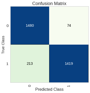
In the positive class, we have 1419 correct predictions and 213 wrong predictions. We can also display the percentages instead of numbers by setting the percent parameter as True.
在肯定类中,我们有1419个正确的预测和213个错误的预测。 通过将percent参数设置为True,我们也可以显示百分比而不是数字。
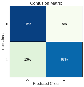
The model performs better on the negative class which is not what we want. One way to achieve this is to tell the model that “positive class (1) is more important than the negative class (0)”. With our random forest classifier, it can be achieved by the class_weight parameter.
该模型在否定类上表现更好,这不是我们想要的。 实现此目的的一种方法是告诉模型“正类(1)比负类(0)更重要”。 使用我们的随机森林分类器,可以通过class_weight参数实现。
Another tool to evaluate the performance of a classification model is ROC (receiver operating characteristics) curve and AOC (area under the curve).
评估分类模型性能的另一个工具是ROC(接收机工作特性)曲线和AOC(曲线下的面积)。
ROC curve summarizes the performance by combining confusion matrices at all threshold values. AUC turns the ROC curve into a numeric representation of performance for a binary classifier. AUC is the area under the ROC curve and takes a value between 0 and 1. AUC indicates how successful a model is at separating positive and negative classes.
ROC曲线通过组合所有阈值处的混淆矩阵来总结性能。 AUC将ROC曲线转化为二进制分类器性能的数字表示。 AUC是ROC曲线下的面积,取值介于0到1之间。AUC表示模型在分离阳性和阴性类别方面的成功程度。
from yellowbrick.classifier import ROCAUCplt.figure(figsize=(10,6))
plt.title("ROC Curve and AUC", fontsize=18)
plt.xlabel("False Positive Rate", fontsize=16)
plt.ylabel("True Positive Rate", fontsize=16)visualizer = ROCAUC(rf, classes=["Not-churned", "Churned"])
visualizer.fit(X_train, y_train)
visualizer.score(X_test, y_test)plt.legend()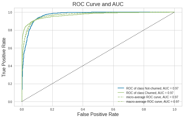
ROC curve gives as an overview of model performance at different threshold values. AUC is the area under the ROC curve between (0,0) and (1,1) which can be calculated using integral calculus. AUC basically aggregates the performance of the model at all threshold values. The best possible value of AUC is 1 which indicates a perfect classifier. AUC is zero if all the predictions are wrong.
ROC曲线概述了在不同阈值下的模型性能。 AUC是ROC曲线下(0,0)与(1,1)之间的面积,可以使用积分计算。 AUC基本上汇总了所有阈值下的模型性能。 AUC的最佳可能值为1,这表示一个完美的分类器。 如果所有预测都错误,则AUC为零。
When it comes to imbalanced datasets, precision or recall is usually the choice of evaluation metric.
对于不平衡的数据集, 精度或召回率通常是评估指标的选择。
The focus of precision is positive predictions. It indicates how many of the positive predictions are true.
精度的重点是积极的预测 。 它表明有多少积极预测是正确的。
The focus of recall is actual positive classes. It indicates how many of the positive classes the model is able to predict correctly.
召回的重点是实际的正面课堂 。 它指示模型能够正确预测多少个肯定类别。
Note: We cannot try to maximize both precision and recall because there is a trade-off between them. Increasing precision decreases recall and vice versa. We can aim to maximize precision or recall depending on the task.
注意 :我们无法尝试同时提高精度和查全率,因为它们之间需要权衡。 提高精度会降低召回率,反之亦然。 我们可以根据任务最大化精度或召回率。
Yellowbrick also offers the Precision-Recall curve which shows the tradeoff between precision and recall.
Yellowbrick还提供了Precision-Recall曲线,该曲线显示了精度和召回率之间的权衡。
from yellowbrick.classifier import PrecisionRecallCurveplt.figure(figsize=(10,6))
plt.title("Precision-Recall Curve", fontsize=18)
plt.xlabel("Recall", fontsize=16)
plt.ylabel("Precision", fontsize=16)viz = PrecisionRecallCurve(rf)
viz.fit(X_train, y_train)
viz.score(X_test, y_test)
plt.legend(loc='lower right', fontsize=12)
After some point, increasing recall causes precision to drop significantly.
在某一点之后,增加的查全率会导致精度大大降低。
Yellowbrick also provides the following visualizations that are useful in evaluating classification models:
Yellowbrick还提供了以下可视化效果,可用于评估分类模型:
- Classification report 分类报告
- Class Prediction Error 类预测错误
- Discrimination Threshold (Only for binary classification) 区分阈值(仅用于二进制分类)
Using informative visualization in the process of evaluating your model will provide you with lots of insights. It will lead you towards improving your model in an efficient way.
在评估模型的过程中使用信息可视化将为您提供许多见解。 它将引导您以有效的方式改进模型。
Instead of just looking at numbers, try to use different approaches to evaluate and thus improve your models.
不仅要查看数字,还应尝试使用不同的方法进行评估,从而改善模型。
Thank you for reading. Please let me know if you have any feedback.
感谢您的阅读。 如果您有任何反馈意见,请告诉我。
机器学习可视化


 325
325

 被折叠的 条评论
为什么被折叠?
被折叠的 条评论
为什么被折叠?
 到【灌水乐园】发言


