准确性可视化：有监督的机器学习分类算法

内部AI (Inside AI)

Measuring the prediction accuracy of any regression or classification algorithm is vital in different stages during modelling and also when the model is live in production.

在建模期间的不同阶段以及在模型投入生产时，测量任何回归或分类算法的预测准确性至关重要。

We have several ways to measure the accuracy of classification algorithms. In the Scikit-learn package, we have several scores like recall score, accuracy score etc. and then we have out of box summarised reports. In my view, most of these metrics have one or more limitations related to verbosity and difficult to understand, potential chance to misinterpret the accuracy in case of imbalance classes in the dataset, need to refer few of the scores to get holistic view etc.

我们有几种方法来衡量分类算法的准确性。 在Scikit-learn程序包中，我们有多个得分，如召回得分，准确性得分等，然后我们提供了现成的摘要报告。 在我看来，这些度量标准中的大多数都有一个或多个与冗长性相关的局限性，并且难以理解，如果数据集中的类别不平衡，则可能会误解准确性，需要引用很少的分数以获得整体视图等。

To better understand the limitation, let us consider the example shown in the table. We have few parameters related to a sample of people and whether they are COVID positive. As we have more people who are COVID negative than people who are infected with the virus hence, I have considered a similar distribution in this example.

为了更好地理解限制，让我们考虑下表中显示的示例。 我们很少有与人群样本以及他们是否为COVID阳性有关的参数。 因此，由于COVID阴性的人比感染病毒的人多，因此在此示例中我考虑了类似的分布。

Imaginary Sample Data For Explanation

虚构样本数据以供解释

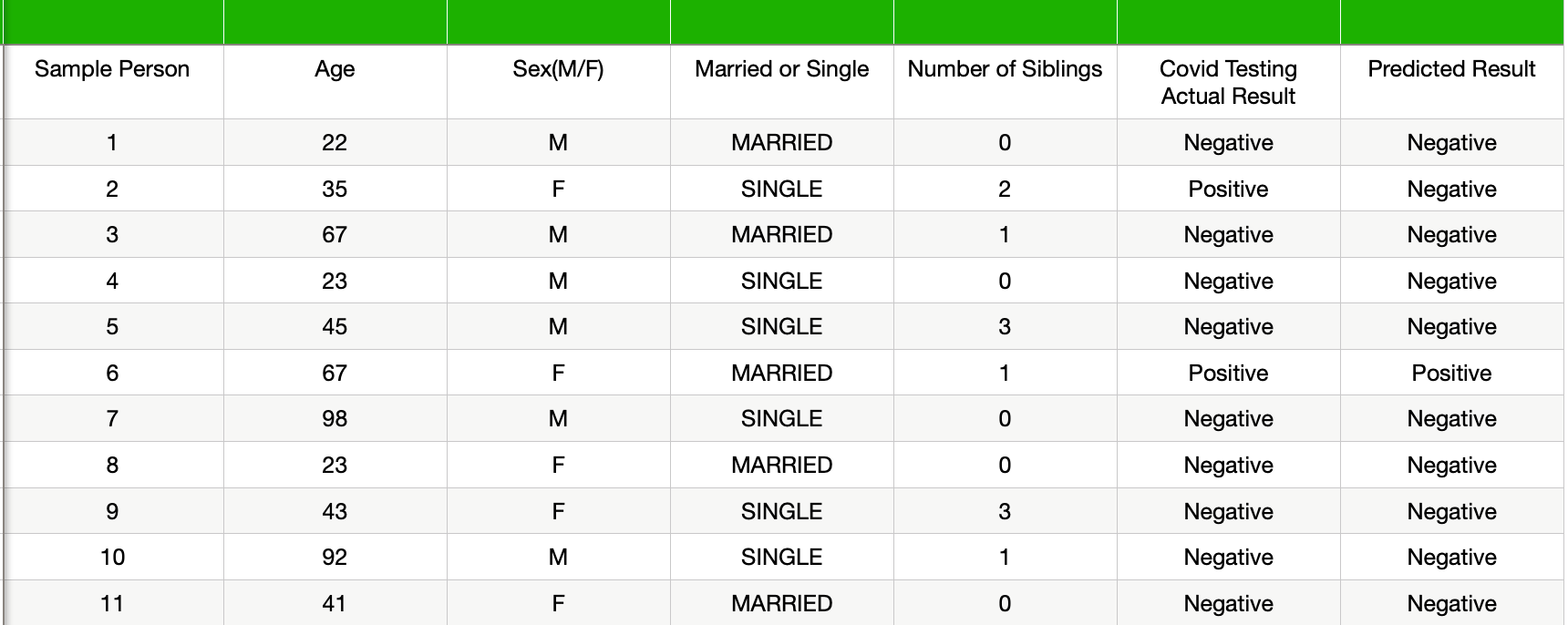
A classification algorithm trained on this datasets predicted the results as shown in the last column. The accuracy score of the classification model is close to 90 per cent. It gives us the impression that the model is quite good at predicting the result.

如上一列所示，在该数据集上训练的分类算法可以预测结果。 分类模型的准确性得分接近90％。 它给我们的印象是该模型非常擅长预测结果。

from sklearn.metrics import recall_score
from sklearn.metrics import classification_report
from sklearn.metrics import accuracy_score# 0- Healthy , 1-  Covidy_true = [0, 1, 0,0,0, 1,0,0,0,0,0]
y_pred = [0, 0, 0,0,0, 1,0,0,0,0,0]print("The recall Score is" , recall_score(y_true, y_pred))
print("The accurracy score is" , accuracy_score(y_true, y_pred))

In reality, the model could predict the COVID positive cases with only 50 per cent times. Deploying such a model only based on one metric or without understanding the areas in which the classification model is making an error can be quite costly.

实际上，该模型只能预测COVID阳性病例的50％。 仅基于一个度量标准或不了解分类模型在其中出错的区域来部署这种模型可能会非常昂贵。

We can make a full sense of the model fit for production usage after considering both the recall and accuracy score and business use case.

在考虑召回率和准确性得分以及业务用例之后，我们可以充分了解适合生产使用的模型。

A visual metric, like the confusion matrix, outshines other metrics in several ways. We get an instant view on the model performance in terms of classification areas the model excelled and the areas which require fine-tuning. Based on the business use case, we can judge quickly from the false positive, false negative, true positive and true negative counts whether the model is ready for deployment.

视觉指标(如混淆矩阵)在几种方面优于其他指标。 我们从模型擅长的分类区域和需要微调的区域方面即时了解模型性能。 根据业务用例，我们可以从误报，误报，真正和真负数快速判断模型是否已准备好进行部署。

Let us learn to visualise and interpret the result of LinearSVCand LogisticRegression with confusion matrix.

让我们学习使用混淆矩阵来可视化和解释LinearSVC和LogisticRegression的结果。

Step 1: We will use the Scikit-learn inbuilt dataset WINE in this article for discussion and Matplotlib for visualisation. In the below code, we have imported the modules which we will be using in our program.

步骤1：我们将使用Scikit-本文中学习内置数据集WINE进行讨论，并使用Matplotlib进行可视化。 在下面的代码中，我们导入了将在程序中使用的模块。

from sklearn.datasets import load_wine
from sklearn.model_selection import train_test_split
from sklearn.preprocessing import StandardScaler 
from sklearn.linear_model import LogisticRegression
from sklearn.svm import LinearSVC
import matplotlib.pyplot as plt
from sklearn.metrics import plot_confusion_matrix

Step 2: The features ( attributes) in the Wine datasets divided into independent and dependent variables. Independent (input features) variables denoted by “X” and the dependent variable is denoted by “y”. Using the method train_test_split is divided into training and testing set.

步骤2： Wine数据集中的特征(属性)分为独立变量和因变量。 用“ X”表示的独立(输入要素)变量和用“ y”表示的因变量。 使用方法train_test_split分为训练集和测试集。

X,y = load_wine(return_X_y=True)X_train, X_test, y_train, y_test = train_test_split(X, y, test_size=0.10,random_state=0)

Step 3: Most of the supervised algorithms in sklearn require standard normally distributed input data centred around zero and have variance in the same order. As the independent variable values in the WINE dataset have a different scale, hence we need to scale it before using it in modelling.

步骤3： sklearn中的大多数监督算法都需要以0为中心的标准正态分布输入数据，并且具有相同顺序的方差。 由于WINE数据集中的自变量值具有不同的比例，因此我们需要在建模之前对其进行缩放。

If you would like to learn more about scaling the independent variables and different scalers in Scikit-learn package, then please refer my article Feature Scaling — Effect Of Different Scikit-Learn Scalers: Deep Dive.

如果您想了解更多有关在Scikit-learn软件包中缩放自变量和不同缩放器的信息 ，请参阅我的文章Feature Scaling —不同Scikit-Learn缩放器的影响：深入研究 。

SC_X=StandardScaler()
X_train_Scaled=SC_X.fit_transform(X_train)
X_test=Scaled=SC_X.transform(X_test)

Step 4: In the below code, a list of classifiers defined along with parameters

步骤4：在下面的代码中，定义了分类器的列表以及参数

classifiers=[ LinearSVC(dual=False),LogisticRegression(solver="liblinear",max_iter=100)]

Step 5: Each classifier is used to train the model in sequence, and the confusion matrix is plotted based on the actual and predicted dependent variable value in the training set.

步骤5：每个分类器用于依次训练模型，并基于训练集中的实际和预测因变量值绘制混淆矩阵。

for clf in classifiers:
    clf.fit(X_train, y_train)
    y_pred = clf.predict(X_test)
    fig=plot_confusion_matrix(clf, X_test, y_test, display_labels=["Bad Wine","Fair Wine","Good Wine"])
    fig.figure_.suptitle("Confusion Matrix for  " + str(clf))
    plt.show()

At first glance itself, we can see that the summation of figures from top left to bottom right diagonal is higher in Linear SVC compare to Logistics regression. It immediately suggests that Linear SVC performed better it identifying the true positive records.

乍一看，我们可以看到，与物流回归相比，线性SVC中左上角到右下角对角线的总和更高。 它立即表明，Linear SVC在识别真实阳性记录方面表现更好。

Confusion Matrix based on the code discussed in the article

基于本文讨论的代码的混淆矩阵

Different metric scores can indicate the accuracy, but with confusion matrix, we can immediately see the classes which the algorithm is misclassifying. In the current example, both the classifiers missed in classifying most of the bad wines accurately. This level of detail information helps to perform focus fine-tuning of the model.

不同的度量分数可以指示准确性，但是使用混淆矩阵，我们可以立即看到算法分类错误的类别。 在当前示例中，两个分类器都未能准确地对大多数劣质葡萄酒进行分类。 此级别的详细信息有助于执行模型的焦点微调。

We have seen that the confusion matrix provides finer details about the classification model prediction pattern for different classes in a nice crisp way. In a single confusion matrix, We can get the details like false alarms (false positive) and correct rejection rates and decide whether the model is acceptable based on the business case.

我们已经看到，混淆矩阵以一种清晰的方式提供了有关不同类的分类模型预测模式的更详细的信息。 在一个混乱的矩阵中，我们可以获得错误警报(误报)和更正拒绝率之类的详细信息，并根据业务案例确定模型是否可以接受。

翻译自: https://towardsdatascience.com/accuracy-visualisation-supervised-machine-learning-classification-algorithms-af13d18fcc6c