


Optimisation is used for a number of day-to-day activities from finding the quickest route to our destination using google maps to ordering food through an online app. In this post, we will go through price optimisation for two main types of loss functions i.e. convex and non-convex. We will also cover the best ways to solve these problems using a python library called scipy. The details of the example data and code used in this blog can be found in this notebook.
优化用于许多日常活动,从使用Google地图找到到达我们目的地的最快路线到通过在线应用程序订购食物。 在这篇文章中,我们将针对两种主要损失函数进行价格优化,即凸函数和非凸函数。 我们还将介绍使用名为scipy的python库解决这些问题的最佳方法。 在此笔记本中可以找到本博客中使用的示例数据和代码的详细信息。
凸优化 (Convex Optimisation)
A convex optimisation problem is a problem where all of the constraints are convex functions, and the objective is a convex function if minimising, or a concave function if maximising. A convex function can be described as a smooth surface with a single global minimum. Example of a convex function is as below:
凸优化问题是所有约束都是凸函数的问题,如果最小化,则目标是凸函数,如果最大化,则目标是凹函数。 凸函数可以描述为具有单个全局最小值的光滑表面。 凸函数的示例如下:
F(x,y) = x2 + xy + y2.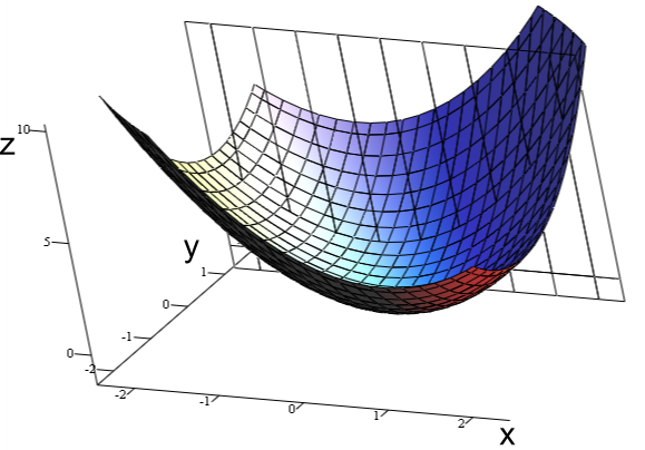
1.数据生成 (1. Data Generation)
In order to look at how optimisation works, I am generating a toy data set, which consists of price, volume and cost. Let’s set the objective of the data set is to find a price that would maximise the total profit.
为了查看优化的工作原理,我正在生成一个玩具数据集,该数据集包括价格,数量和成本。 让我们设置数据集的目标是找到可以使总利润最大化的价格。
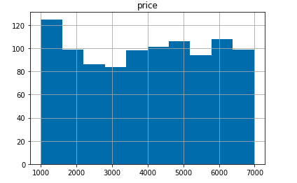
Price: This is a random number generated between 1000 and 7000. The data is generated using numpy random function.
价格:这是一个介于1000和7000之间的随机数。数据是使用numpy随机函数生成的。
Volume: volume is generated as a straight line function of price with a declining slope as shown below:
交易量:交易量是价格的直线函数,其斜率下降,如下所示:
f(volume) = (-price/2)+4000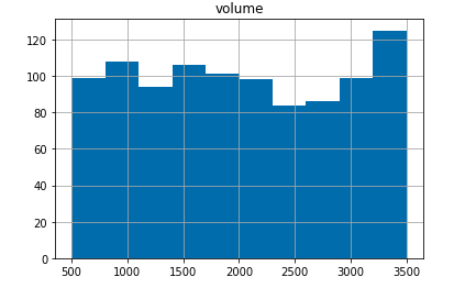
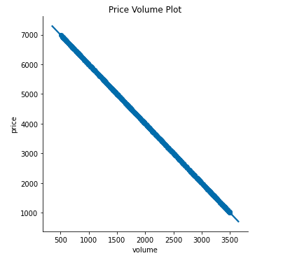
The relationship between price and volume is as shown below. As expected we see an increase in volume of products sold as the price decreases.
价格和数量之间的关系如下所示。 正如预期的那样,随着价格下降,我们看到销售产品的数量有所增加。
Cost: The cost variable represent the cost of manufacturing of the product. This takes into account some fixed costs (i.e. 300) and a variable costs which is a function of volume (i.e. 0.25).
成本:成本变量代表产品的制造成本。 这考虑了一些固定成本(即300)和可变成本(其是数量的函数)(即0.25)。
f(cost) = 300+volume*0.25Now that we have all the variables that we need, we can use the simple formula below to calculate profit:
现在我们有了所需的所有变量,我们可以使用以下简单公式来计算利润:
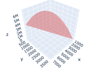
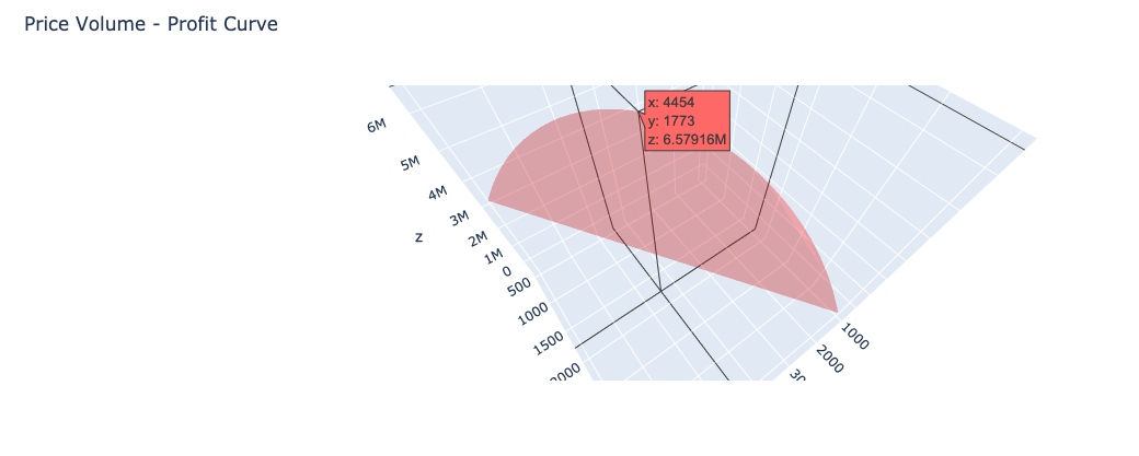
f(profit) = (price — cost)*volumeA 3-D plot of the price, volume and profit is as shown below. We can see that it is a bell shaped curve with a peak profit at a particular volume and cost. A objective for a business may be to maximise profit and in the following section’s I will show how we can achieve this using scipy.
价格,数量和利润的3-D图如下所示。 我们可以看到这是一个钟形曲线,在特定的数量和成本下利润达到峰值。 企业的目标可能是使利润最大化,在下面的部分中,我将说明如何使用scipy来实现这一目标。
2.根据观测数据估算成本和数量 (2.Estimate cost and volume from observational data)
In the above section we have generated a sample data set. However in the real world we may have access to a small set of observations i.e. price, volume and costs for a product. Additionally we will not know the underlying function which governs the relationship between the dependent and independent variable.
在上一节中,我们生成了一个样本数据集。 但是,在现实世界中,我们可能会获得少量观察结果,即产品的价格,数量和成本。 另外,我们将不知道控制因变量和自变量之间关系的基础功能。
In order to simulate observational data let’s take a cut of the generated data i.e. all points where the price is “<3000”. With this observational data we need to find the relationship between price vs cost and volume vs cost. We can do that by performing a simple linear regression on the observation data set. However for real world problem this may involve building complex non-linear models with a large number of independent variables.
为了模拟观测数据,让我们对生成的数据进行裁剪,即价格“ <3000”的所有点。 利用这些观察数据,我们需要找到价格与成本之间以及体积与成本之间的关系。 我们可以通过对观察数据集执行简单的线性回归来做到这一点。 但是,对于现实世界的问题,这可能涉及使用大量自变量构建复杂的非线性模型。
Linear Regression:
线性回归:
Price vs Volume
价格与数量
We take price as an independent variable ‘X’ and volume as a dependent variable ‘y’. Using the stats model library in python, we can determine a linear regression model to capture the relationship between volume and price.
我们将价格作为自变量“ X”,将数量作为因变量“ y”。 使用python中的统计模型库,我们可以确定线性回归模型来捕获数量和价格之间的关系。
As seen below from the observational data we are achieving a R-squared of 1 (i.e. 100%), which means the change in volume is perfectly explained by the change in price for the product. However this perfect relationship will rarely be observable in real-life data sets.
从观察数据中可以看出,我们实现的R平方为1(即100%),这意味着产品价格的变化可以完美地说明体积的变化。 但是,这种完美的关系在现实生活的数据集中很难被观察到。
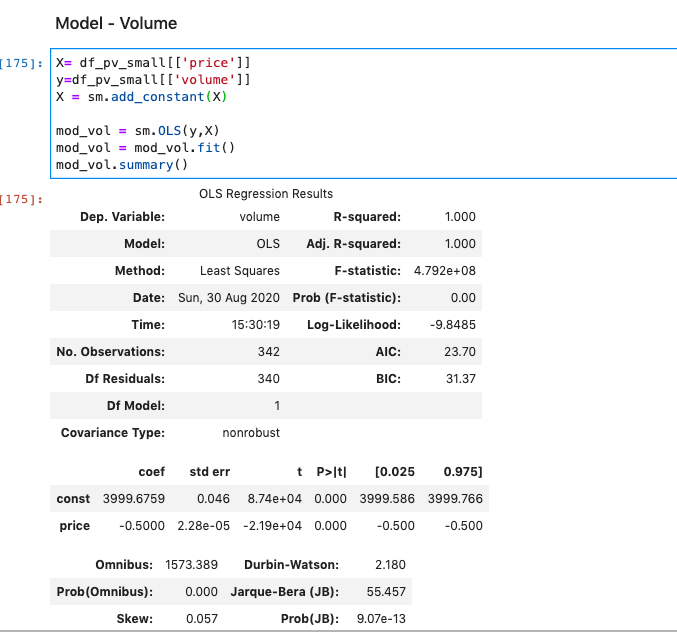
Additionally we can see the bias of -3,999.67 and the coefficient of -0.5 for prices approximates the function used to generate the volume data.
另外,我们可以看到-3,999.67的偏差和-0.5的价格系数近似于用于生成数量数据的函数。
2. Volume vs Cost
2.数量与成本
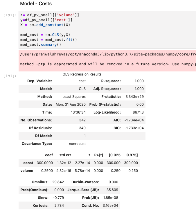
In a similar manner a linear regression with cost as the dependent variable ‘y’ and volume as the independent variable ‘X’ is performed below. We can see that the bias and co-efficient for the cost model approximates the function used to generate the cost data. Hence we can now use these trained models to determine cost and volume for the convex optimisation.
以类似的方式,下面执行线性回归,其中成本为因变量“ y”,数量为自变量“ X”。 我们可以看到,成本模型的偏差和系数近似于用于生成成本数据的函数。 因此,我们现在可以使用这些训练有素的模型来确定凸优化的成本和数量。
使用scipy进行优化 (Optimisation using scipy)
We will use the scipy optimise library for the optimisation. The library has a minimise function, which takes in the below parameters, additional details on the scipy minimise function can be found here:
我们将使用scipy优化库进行优化。 该库具有最小化函数,该函数接受以下参数,有关scipy最小化函数的更多详细信息,请参见此处 :
result = optimize.minimize(fun=objective,
                           x0=initial,
                           method=’SLSQP’,
                           constraints=cons,
options={‘maxiter’:100, ‘disp’: True})fun:The objective function to be minimised. In our case we want to maximise the profit. Hence that would mean minimisation of ‘-profit’, where profit is calculate as: profit = (price — cost)*volume
fun:目标函数被最小化。 在我们的案例中,我们希望最大化利润。 因此,这将意味着“利润”的最小化,其中利润的计算方式为: 利润=(价格-成本)*数量
def cal_profit(price):
 volume = mod_vol.predict([1, price])
 cost = mod_cost.predict([1, volume])
 profit = (price — cost)*volume
 return profit###### The main objective function for the minimisation.
def objective(price):
 return -cal_profit(price)
2. x0: Initial guess i.e in this case we are setting an initial price of 2,000.
2. x0:初始猜测,即在这种情况下,我们将初始价格定为2,000。
initial = [2000]3. bounds: Bounds are the lower and upper limit intervals to be used in the optimisation. It can be set only for for certain optimisation methods which supports bounded inputs such as L-BFGS-B, TNC, SLSQP, Powell, and trust-constr methods.
3.界限:界限是优化中使用的下限和上限区间。 只能为某些支持有界输入的优化方法(例如L-BFGS-B,TNC,SLSQP,Powell和trust-constr方法)设置此属性。
#################### bounds ####################
bounds=([1000,10000])
4. constraints: Here we are specifying constraints to the optimisation problem. The constraints in this case is the volume of products that can be produced (i.e. setting this to 3,000 units). It is an inequality constraint i.e. the volume has to be less than the specified number of units. Other types of constrains such as equality constraints are also available for use.
4.约束:这里我们指定优化问题的约束。 在这种情况下,约束条件是可以生产的产品数量(即,将其设置为3,000个单位)。 这是一个不平等约束,即体积必须小于指定的单位数。 其他类型的约束(例如相等约束)也可以使用。
# Left-sided inequality from the first constraint
def constraint1(price):
    return 3000-mod_vol.predict([1, price])# Construct dictionaries
con1 = {'type':'ineq','fun':constraint1}# Put those dictionaries into a tuple
cons = (con1)5. methods: There a number of methods available for performing the minimisation operation e.g. (see reference):
5 。 方法 :有许多方法可用于执行最小化操作,例如(请参阅参考资料 ):
‘Nelder-Mead’ (see here)
“内德米德” (请参阅此处)
‘BFGS’ (see here)
'BFGS' (请参阅此处)
‘Newton-CG’ (see here)
“牛顿-CG” (请参阅此处)
‘L-BFGS-B’ (see here)
'L-BFGS-B' (请参阅此处)
‘SLSQP’ (see here)
'SLSQP' (请参阅此处)
‘trust-constr’(see here)
'trust-constr' (请参阅此处)
We will use the SLSQP method for optimisation. Sequential quadratic programming (SQP or SLSQP) is an iterative method for constrained nonlinear optimisation.
我们将使用SLSQP方法进行优化。 顺序二次规划 ( SQP或SLSQP )是用于约束非线性优化的迭代方法。
Not all of the above methods support the use of both bounds and constraints. Hence we are using SLSQP, which supports the use of both the bounds and constraints for optimisation.
并非所有上述方法都支持界限和约束的使用。 因此,我们正在使用SLSQP,它支持使用边界和约束进行优化。
凸优化的结果 (Results of convex optimisation)
The optimisation was run for a total of 3 iterations. Based on this the objective function has returned a value of -6.6 mil (i.e. -6,587,215.16). This results in a price of 4,577 and volume of 1,710. We are getting a negative value because we are maximising for profit by minimising for negative profit, which is a convex function.
该优化总共运行了3次迭代。 基于此,目标函数返回的值为-6.6百万(即-6,587,215.16)。 这导致价格为4,577和数量为1,710。 我们之所以得到负值,是因为我们通过使负利润最小化来最大化利润,这是一个凸函数。
Optimization terminated successfully.    (Exit mode 0)
            Current function value: -6587215.163007045
            Iterations: 3
            Function evaluations: 9
            Gradient evaluations: 3
The results of the optimisation closely matches to the maximum profit as seen in the generated data set. Hence we know that the optimisation has worked as expected.
从生成的数据集中可以看出,优化的结果与最大利润紧密匹配。 因此,我们知道优化已按预期进行。
非凸优化 (Non Convex Optimisation)
In most of the machine learning problems we come across loss surfaces which are non-convex in nature. Hence they will have multiple local minimum. Hence while solving for such non-convex problems it may be simpler and less computationally intensive if we “convexify” a problem (make it convex optimisation friendly), then to use non-convex optimisation. I will demonstrate how we can achieve this through the below example.
在大多数机器学习问题中,我们遇到的损失表面实际上是非凸的。 因此,它们将具有多个局部最小值。 因此,在解决此类非凸问题时,如果我们将一个问题“凸化” (使其友好地凸优化) ,然后使用非凸优化,则可能会更简单且计算量更少。 我将通过以下示例演示如何实现此目标。
非凸数据集生成: (Non convex data set genration:)
Here we have created another product with a slightly different price, volume and profit profile. Let’s say that the company can produce only one of these products and wants to use optimisation to find out which of the products it needs to focus on and what price it needs to sell it at.
在这里,我们创建了另一种产品,其价格,数量和利润情况略有不同。 假设该公司只能生产其中一种产品,并且想使用优化来找出需要关注的产品以及以什么价格出售产品。
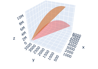
使用凸极小化处理非凸数据 (Use of Convex minimisation for non-convex data)
For the above data if we use the same convex optimisation as above, the solution we get will be a local minimum as seen below. We get a max profit of 6.86 mil for a optimised price of 5, 018 and product type 0.
对于上述数据,如果我们使用与上述相同的凸优化,则得到的解将是局部最小值,如下所示。 我们以最优价格5 018和产品类型0获得最大利润686万 。

跳台算法 (Basinhopping algorithm)
Basin-hopping is an algorithm that combines a global stepping algorithm along with a local minimisation at each step. Hence this can be used to seek the best of all the local minimum options available for the non-convex loss surface. The below code demonstrates the implementation of this algorithm.
盆地跳跃是一种将全局步进算法与每个步骤的局部最小化相结合的算法。 因此,这可用于在非凸面损耗的所有局部最小选项中寻求最佳。 下面的代码演示了该算法的实现。
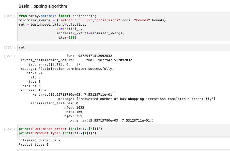
As seen above we have use the same method i.e. SLSQP and the same bounds and constraints as the previous example. However, we now get a slightly different result. The maximum profit is 9.8 mil with an optimised price of 5,957 and product type of 1.
如上所示,我们使用与前面的示例相同的方法,即SLSQP以及相同的边界和约束。 但是,我们现在得到的结果略有不同。 最大利润为980万 ,优化价格为5957 ,产品类型为1 。
结论: (Conclusion:)
In summary, we have reviewed the use of optimisation libraries in scipy for a simple convex optimisation data-set which has a single global minimum and also reviewed the use of basin-hopping algorithm in cases where the loss surface has multiple local minimum and a global minimum. Hope you find the above post useful and the framework provided to solve optimisation problems in the real world.
总之,对于具有单个全局最小值的简单凸优化数据集,我们已经审查了在scipy中使用优化库的情况,并且在损失面具有多个局部最小值和全局损失的情况下,也回顾了盆地跳跃算法的使用。最低。 希望以上文章对您有用,并为解决现实世界中的优化问题提供了框架。
翻译自: https://medium.com/@prajwalshreyas/convex-and-non-convex-optimisation-899174802b60


 475
475

 被折叠的 条评论
为什么被折叠?
被折叠的 条评论
为什么被折叠?
 到【灌水乐园】发言


