


 本文介绍了Python中计算Pearson相关系数的方法,用于量化两个数据集之间的关系。通过实例展示了数据集1、2、3的散点图,解释了如何根据数据的分布估算ρ的值。还强调了相关性并不意味着因果关系,并提供了计算协方差、方差和标准偏差的代码实现,以帮助理解相关性的计算和意义。
Correlation is the process of quantifying the relationship between two sets of values, and in this post I will be writing code in Python to calculate possibly the best-known type of correlation — the Pearson Correlation Coefficient.
关联是量化两组值之间关系的过程,在这篇文章中,我将用Python编写代码来计算可能最著名的关联类型-Pearson关联系数。
相关概述 (An Overview of Correlation)
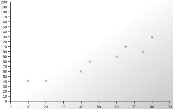
Consider the following three data sets and their graphs, or, more accurately, scatter plots. The x-axis represents an independent variable, and the y-axis represents a dependent variable, ie. one which we believe may change as a result of changes in the independent variable.
请考虑以下三个数据集及其图形,或更准确地说,是散点图。 x轴表示自变量, y轴表示因变量,即。 我们认为可能会由于自变量的变化而发生变化。
数据集1 (Data Set 1)
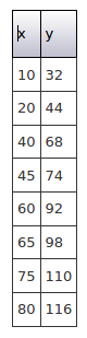

In this data set all the points are on a straight line — there is clearly a relationship between them.
在此数据集中,所有点都在一条直线上-显然它们之间存在关系。
数据集2 (Data Set 2)
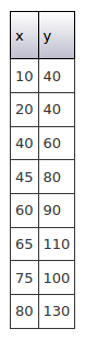
Here the data is a bit more scattered but there is still a clear relationship, subject to some minor fluctuations.
这里的数据较为分散,但仍然存在明确的关系,但会受到一些轻微的波动的影响。
数据集3 (Data Set 3)
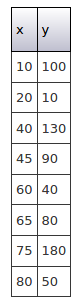

In this last set of data the points appear completely random, with little or no relationship between x and corresponding y values.
在这最后一组数据中,这些点看起来完全是随机的,x与相应的y值之间几乎没有关系。
量化关系 (Quantifying the Relationships)
Relationships within bivariate data such as the examples above can be precisely quantified by calculating the Pearson Correlation Coefficient, usually referred to as ρ, the Greek letter rho. This gives us a number between -1 and 1, -1 being a perfect negative correlation (ie as the independent variable increases the dependent variable decreases, so the line runs top-left to bottom-right) and 1 being a perfect positive correlation (ie both variables increase and the line runs bottom-left to top-right). Values in between represent various degrees of imperfect correlation, with 0 being none at all.
可以通过计算Pearson相关系数 (通常称为ρ ,希腊字母rho)来精确地量化双变量数据中的关系(例如上述示例)。 这给了我们一个介于-1和1之间的数字,-1是一个完美的负相关性(即,随着自变量的增加,因变量减小,因此该行从左上到右下),而1是一个完美的正相关性(即两个变量都增加,并且该行从左下到右上)。 介于两者之间的值表示不同程度的不完全相关,其中0根本没有。
As rough estimates, in Data Set 1 we would expect ρ to be 1, in Data Set 2 we would expect ρ to be around 0.9, and in Data Set 3 ρ would be close to 0.
粗略估计,在数据集1中,我们期望ρ为1,在数据集2中,我们期望ρ约为0.9,而在数据集3中, ρ接近于0。
Full details of the Pearson Correlation Coefficient are on Wikipedia. In short the formula is:
皮尔逊相关系数的完整细节在维基百科上 。 简而言之,公式为:
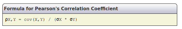
cov is the covariance of the paired data, and σ is the standard deviation of the individual sets of data. These will be explored as we get to them.
cov是配对数据的协方差,而σ是各个数据集的标准偏差。 这些将在我们到达它们时进行探讨。
警告 (Caveat)
There is a famous phrase in statistics: “correlation does not imply causation”. A strong correlation between two variables might just be by chance, even where common sense might make you believe the association could be genuine. A strong correlation should only ever be used as a basis for further investigation, particularly in this age of Big Data number crunching where seemingly unrelated data sets can be compared quickly and cheaply.
在统计中有一个著名的短语:“相关并不意味着因果关系”。 即使常识可能使您相信关联可能是真实的,两个变量之间的强关联也可能只是偶然而已。 强烈的相关性仅应用作进一步研究的基础,尤其是在这个大数据数量紧缩的时代,在这个时代看似无关的数据集可以快速而廉价地进行比较。
There are many examples of datasets which appear to exhibit strong but obviously coincidental correlation. Many of these are flippant or humorous, a well-known one being a correlation between sightings of storks and the number of babies “delivered” in a town in Germany. Now you know why I chose that header image!
有许多数据集示例似乎表现出很强的但很明显的巧合相关性。 其中许多是轻率的或幽默的,众所周知的是,在德国的一个小镇上,发现鹳鸟与“分娩”的婴儿数量之间存在相关性。 现在您知道我为什么选择该标题图像了!
编码 (Coding)
This project consists of these files…
该项目包含以下文件...
- pearsoncorrelation.py 皮尔逊相关系数
- data.py data.py
- main.py main.py
…which you can clone or download from Github.
…您可以从Github克隆或下载。
This is the first file.
这是第一个文件。
import math


def pearson_correlation(independent, dependent):


    """
    Implements Pearson's Correlation, using several utility functions to
    calculate intermediate values before calculating and returning rho.
    """


    # covariance
    independent_mean = _arithmetic_mean(independent)
    dependent_mean = _arithmetic_mean(dependent)
    products_mean = _mean_of_products(independent, dependent)
    covariance = products_mean - (independent_mean * dependent_mean)


    # standard deviations of independent values
    independent_standard_deviation = _standard_deviation(independent)


    # standard deviations of dependent values
    dependent_standard_deviation = _standard_deviation(dependent)


    # Pearson Correlation Coefficient
    rho = covariance / (independent_standard_deviation * dependent_standard_deviation)


    return rho


def  _arithmetic_mean(data):


    """
    Total / count: the everyday meaning of "average"
    """


    total = 0


    for i in data:
        total+= i


    return total / len(data)


def  _mean_of_products(data1, data2):


    """
    The mean of the products of the corresponding values of bivariate data
    """


    total = 0


    for i in range(0, len(data1)):
        total += (data1[i] * data2[i])


    return total / len(data1)


def  _standard_deviation(data):


    """
    A measure of how individual values typically differ from the mean_of_data.
    The square root of the variance.
    """


    squares = []


    for i in data:
        squares.append(i ** 2)


    mean_of_squares = _arithmetic_mean(squares)
    mean_of_data = _arithmetic_mean(data)
    square_of_mean = mean_of_data ** 2
    variance = mean_of_squares - square_of_mean
    std_dev = math.sqrt(variance)


    return std_dev
Most of the work done by pearson_correlation is delegated to other functions, which calculate various intermediate values needed to actually calculate the correlation coefficient. Firstly we need the arithmetic means of both sets of data, and the mean of the products of the twin datasets. Next we calculate the covariance.
pearson_correlation完成的大部分工作都委托给其他函数,这些函数计算实际计算相关系数所需的各种中间值。 首先,我们需要两组数据的算术平均值以及孪生数据集乘积的平均值。 接下来,我们计算协方差。
Covariance is a rather complex concept which you might like to look into on Wikipedia or elsewhere, but an easy way to remember how to calculate it is mean of products minus product of means. The mean of products is the mean of each pair of values multiplied together, and the product of means is simply the means of the two sets of data multiplied together.
协方差是一个相当复杂的概念,您可能想在Wikipedia上或其他地方研究一下,但是记住如何计算它的一种简单方法就是乘积减去均值乘积 。 产品的平均值是平均每对值的相乘,和手段的产品简单地是两组数据的手段相乘。
Next we need the standard deviations of the two datasets. Standard deviation can be thought of roughly as the average amount by which the individual values vary from the mean. (It is not that exactly, which is a different figure known as mean of absolute deviation or MAD, but the concepts are similar.) The standard deviation is the square root of the variance which uses squared values to eliminate negative differences.
接下来,我们需要两个数据集的标准偏差。 标准偏差可以粗略地看成是各个值与平均值之间的平均值的平均值。 (不是完全一样,这是一个不同的数字,称为绝对偏差或MAD的平均值,但是概念相似。)标准偏差是方差的平方根,它使用平方值消除负差。
An easy way to remember how to calculate a variance is mean of squares minus square of mean. The mean of squares is simple enough, just square all the values and calculate their mean; and the square of mean is self-explanatory. Once you have calculated the variance don’t forget to calculate its square root to get the standard deviation.
记住如何计算方差的一种简单方法是均方减去均方 。 平方的平均值非常简单,只需对所有值求平方并计算其平均值即可; 均方根是不言而喻的。 一旦计算出方差,就不要忘记计算其平方根以获得标准偏差。
The methods of calculating variance and covariance are similar: if you decide to memorise my phrases don’t mix them up! Here they are again:
计算方差和协方差的方法类似:如果您决定记住我的短语,请不要混淆它们! 他们又来了:
covariance: mean of products minus product of means
协方差:乘积平均值减去均值乘积
variance: mean of squares minus square of mean
方差 : 均方减去均方
Having calculated all the intermediate values we can then use them to implement the formula from above:
计算完所有中间值后,我们可以使用它们来实现上述公式:
The three private functions which follow calculate the arithmetic mean, mean of products and standard deviation. These have wide uses beyond Pearson’s Correlation and could alternatively be implemented as part of a general purpose statistical library.
随后的三个私有函数计算算术平均值,乘积平均值和标准偏差。 这些在Pearson的Correlation之外具有广泛的用途,也可以作为通用统计库的一部分来实现。
Before we try out the above code we need a few pieces of data so I have created a function called populatedata in data.py which returns a list populated with one of the three datasets show above.
在尝试上面的代码之前,我们需要一些数据,因此我在data.py中创建了一个称为populatedata的函数,该函数返回一个填充有上面显示的三个数据集之一的列表。
def populatedata(independent, dependent, dataset):


    """
    Populates two lists with one of three sets of bivariate data
    suitable for testing and demonstrating Pearson's Correlation
    """


    del independent[:]
    del dependent[:]


    if dataset == 1:
        independent.extend([10,20,40,45,60,65,75,80])
        dependent.extend([32,44,68,74,92,98,110,116])
        return True


    elif dataset == 2:
        independent.extend([10,20,40,45,60,65,75,80])
        dependent.extend([40,40,60,80,90,110,100,130])
        return True


    elif dataset == 3:
        independent.extend([10,20,40,45,60,65,75,80])
        dependent.extend([100,10,130,90,40,80,180,50])
        return True


    else:
        return False
Now we can move on to our main function.
现在我们可以继续我们的main功能。
import data
import pearsoncorrelation


def main():


    """
    Iterates the three available sets of data
    and calls function to calculate rho.
    Then prints the data and Pearson Correlation Coefficient.
    """


    print("-------------------------")
    print("| codedrome.com         |")
    print("| Pearson's Correlation |")
    print("-------------------------\n")


    independent = []
    dependent = []


    for d in range(1, 4):


        if data.populatedata(independent, dependent, d) == True:


            rho = pearsoncorrelation.pearson_correlation(independent, dependent)


            print("Dataset %d\n---------" % d)
            print("Independent data: " + (str(independent)))
            print("Dependent data:   " + (str(dependent)))
            print("Pearson Correlation Coefficient rho = %1.2f\n" % rho)
        else:
            print("Cannot populate Dataset %d" % d)


main()
We firstly create a pair of lists and then loop through the three available datasets, populating the lists and calculating the correlation coefficient. Finally the data and correlation are printed.
我们首先创建一对列表,然后遍历三个可用数据集,填充列表并计算相关系数。 最后打印数据和相关性。
We have now finished writing code so can run it with the following command:
现在我们已经完成了代码编写,因此可以使用以下命令运行它:
python3.8 main.py
python3.8 main.py
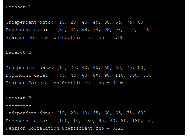
Earlier I gave rough estimates of ρ for the three data sets as 1, 0.9 and 0. As you can see they are actually 1.0, 0.96 and 0.21 to 2dp. You can change the accurancy printed if you wish.
之前,我对三个数据集1、0.9和0给出了ρ的粗略估计。您可以看到它们实际上是1.0、0.96和0.21至2dp。 您可以根据需要更改打印的精度。
“现实世界”中的相关性 (Correlation in the “Real World”)
I have written many articles on implementing various statistical and mathematical processes for purely educational reasons. I strongly believe that the best way to understand any sort of number crunching, be it simple statistics or some sort of sophisticated machine learning algorithm, is to code it from scratch.
我纯粹出于教育的原因写了许多关于实现各种统计和数学过程的文章。 我坚信,无论是简单的统计数据还是某种复杂的机器学习算法,理解任何类型的数字运算的最佳方法就是从头开始编写代码。
If you actually need to calculate a correlation in Python then you would almost certainly use Numpy’s corrcoef function, but I hope that by reading this article you gain a deeper understanding of both how the correlation is calculated and it’s meaning.
如果您实际上需要在Python中计算相关性,那么您几乎可以肯定会使用Numpy的 corrcoef函数,但是我希望通过阅读本文可以对相关性的计算方式及其含义有更深入的了解。
下一步:回归 (Next Step: Regression)
If you have discovered a strong correlation in your data your next step will probably be to put numbers to that relationship by working out the formula of the straight line which best fits the data. That process is called linear regression and will be the subject of a future post.
如果您发现数据中存在很强的相关性,那么下一步可能是通过计算最适合数据的直线公式将数字添加到该关系中。 该过程称为线性回归,将成为未来发布的主题。
翻译自: https://medium.com/python-in-plain-english/pearson-correlation-in-python-a9fc32c3aa82


 3441
3441

 被折叠的 条评论
为什么被折叠?
被折叠的 条评论
为什么被折叠?
 到【灌水乐园】发言


