


已知两点坐标拾取怎么操作
有关深层学习的FAU讲义 (FAU LECTURE NOTES ON DEEP LEARNING)
These are the lecture notes for FAU’s YouTube Lecture “Deep Learning”. This is a full transcript of the lecture video & matching slides. We hope, you enjoy this as much as the videos. Of course, this transcript was created with deep learning techniques largely automatically and only minor manual modifications were performed. Try it yourself! If you spot mistakes, please let us know!
这些是FAU YouTube讲座“ 深度学习 ”的 讲义 。 这是演讲视频和匹配幻灯片的完整记录。 我们希望您喜欢这些视频。 当然,此成绩单是使用深度学习技术自动创建的,并且仅进行了较小的手动修改。 自己尝试! 如果发现错误,请告诉我们!
导航 (Navigation)
Previous Lecture / Watch this Video / Top Level / Next Lecture
Welcome back to deep learning! So today, we want to look into the applications of known operator learning and a particular one that I want to show today is CT reconstruction.
欢迎回到深度学习! 因此,今天,我们要研究已知的操作员学习的应用程序,而我今天要展示的特定应用是CT重建。
So here, you see the formal solution to the CT reconstruction problem. This is the so-called filtered back-projection or Radon inverse. This is exactly the equation that I referred to earlier that has already been solved in 1917. But as you may know, CT scanners have only been realized in 1971. So actually, Radon who found this very nice solution has never seen it put to practice. So, how did he solve the CT reconstruction problem? Well, CT reconstruction is a projection process. It’s essentially a linear system of equations that can be solved. The solution is essentially described by a convolution and a sum. So, it’s a convolution along the detector direction s and then a back-projection over the rotation angle θ. During the whole process, we suppress negative values. So, we kind of also get a non-linearity into the system. This all can also be expressed in matrix notation. So, we know that the projection operations can simply be described as a matrix A that describes how the rays intersect with the volume. With this matrix, you can simply take the volume x multiplied with A and this gives you the projections p that you observe in the scanner. Now, getting the reconstruction is you take the projections p and you essentially need some kind of inverse or pseudo-inverse of A in order to compute this. We can see that there is a solution that is very similar to what we’ve seen in the above continuous equation. So, we have essentially a pseudo-inverse here and that is A transpose times A A transpose inverted times p. Now, you could argue that the inverse that you see here in a is actually the filter. So, for this particular problem, we know that the inverse of A A transpose will form a convolution.
因此,在这里,您将看到CT重建问题的正式解决方案。 这就是所谓的滤波反投影或Radon逆。 这正是我之前提到的方程式,该方程式在1917年已经解决。但是,您可能知道,CT扫描仪直到1971年才实现。因此,实际上,发现这种非常好的解决方案的Radon从未见过将其付诸实践。 。 那么,他是如何解决CT重建问题的呢? 好吧,CT重建是一个投影过程。 从本质上讲,这是一个可以求解的线性方程组。 该解决方案基本上由卷积和和来描述。 因此,它是沿着检测器方向s的卷积,然后是旋转角度θ上的反投影。 在整个过程中,我们抑制负值。 因此,我们也将非线性引入系统中。 所有这些也可以用矩阵符号表示。 因此,我们知道投影操作可以简单地描述为矩阵A ,该矩阵A描述光线与体积的相交方式。 使用此矩阵,您只需将体积x乘以A,就可以得出在扫描仪中观察到的投影p。 现在,要进行重构,您需要获得投影p,并且您实际上需要某种A的逆或伪逆才能进行计算。 我们可以看到,有一个解决方案与上面的连续方程式非常相似。 因此,这里我们基本上有一个伪逆,即A转置时间A A转置反向时间p 。 现在,您可以争辩说,您在a中看到的逆实际上是过滤器。 因此,对于这个特定问题,我们知道AA转置的逆会形成卷积。
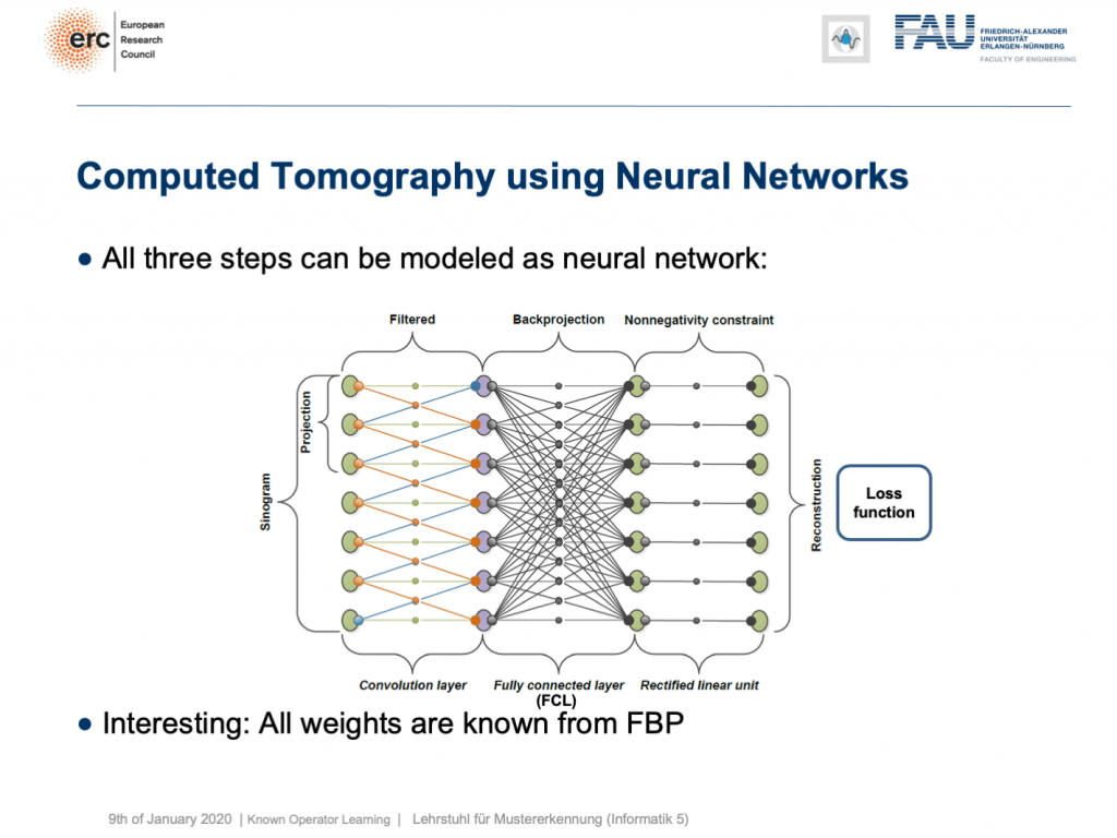
This is nice because we know how to implement convolutions into deep networks, right? Matrix multiplications! So, this is what we did. We can map everything into a neural network. We start on the left-hand side. We put in the Sinogram, i.e., all of the projections. We have a convolutional layer that is computing the filtered projections. Then, we have a back-projection that is a fully connected layer and it’s essentially this large matrix A. Finally, we have the non-negativity constraint. So essentially, we can define a neural network that does exactly filtered back-projection. Now, this is actually not so super interesting because there’s nothing to learn. We know all of those weights and by the way, the matrix A is really huge. For 3-D problems, it can approach up to 65,000 terabytes of memory in floating-point precision. So, you don’t want to instantiate this matrix. The reason why you don’t want to do that it that it’s very sparse. So, only a very small fraction of the elements in A are actual connections. This is very nice for CT reconstruction because then you typically never instantiate A but you compute A and A transpose simply using raytracers. This is typically done on a graphics board. Now, why are we talking about all of this? Well, we’ve seen there are cases where CT reconstruction is insufficient and we could essentially do trainable CT reconstruction.
很好,因为我们知道如何将卷积实现为深度网络,对吗? 矩阵乘法! 因此,这就是我们所做的。 我们可以将所有内容映射到神经网络。 我们从左侧开始。 我们输入了Singram,即所有的预测。 我们有一个卷积层,用于计算滤波后的投影。 然后,我们有一个反投影,它是一个完全连接的层,本质上就是这个大矩阵A。 最后,我们有非负约束。 因此,从本质上讲,我们可以定义一个精确过滤反向投影的神经网络。 现在,这实际上并不是那么有趣,因为没有什么可学的。 我们知道所有这些权重,顺便说一下,矩阵A确实很大。 对于3D问题,它可以以浮点精度接近65,000 TB的内存。 因此,您不想实例化此矩阵。 您不想这样做的原因是它非常稀疏。 因此, A中的元素中只有很小一部分是实际连接。 这对于CT重建非常好,因为您通常从不实例化A,而是仅使用光线跟踪器计算A和A转置。 这通常在图形板上完成。 现在,我们为什么要谈论所有这些? 好吧,我们已经看到了CT重建不足的情况,并且我们基本上可以进行可训练的CT重建。
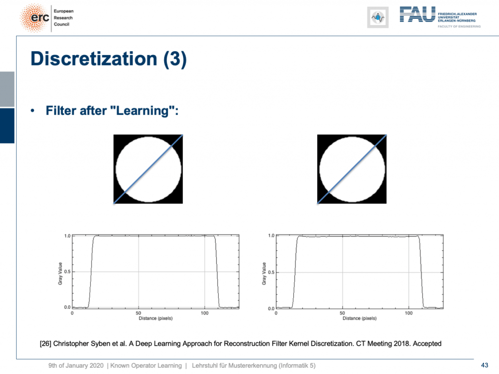
Already, if you look at a CT book, you run into the first problems. If you implement it by the book and you just want to reconstruct a cylinder that is merely showing the value of one within this round area, then you would like to have an image like this one where everything is one within the cylinder and outside of the cylinder it’s zero. So, we’re showing this line plot here along the blue line through the original slice image. Now, if you just implement filtered back-projection, as you find it in the textbook, you get a reconstruction like this one. The typical mistake is that you choose the length of the Fourier transform too short and the other one is that you don’t consider the discretization appropriately. Now, you can work with this and fix the problem in the discretization. So what you can do now is essentially train the correct filter using learning techniques. So, what you would do in a classical CT class is you would run through all the math from the continuous integration to the discrete version in order to figure out the correct filter coefficients.
如果已经看了一本CT书,就会遇到第一个问题。 如果您通过书来实现它,而只想重建一个圆柱体,而该圆柱体仅显示该圆形区域内一个圆柱体的值,那么您将希望获得一个像这样的图像,其中一切都在圆柱体之内和之外。气缸为零。 因此,我们在这里显示此线图,沿着原始切片图像的蓝线。 现在,如果您只是实现滤波后的反投影,就像在教科书中找到的那样,您将获得像这样的重构。 一个典型的错误是您选择傅立叶变换的长度太短,而另一个错误是您没有适当考虑离散化。 现在,您可以使用它并解决离散化问题。 因此,您现在可以做的就是使用学习技术来训练正确的滤波器。 因此,在经典的CT类中,您将经历从连续积分到离散形式的所有数学运算,以便找出正确的滤波器系数。
Instead, here we show that by knowing that it takes the form of convolution, we can express our inverse simply as p times the Fourier transform which is also just a matrix multiplication F. Then, K is a diagonal matrix that holds the spectral weights followed an inverse Fourier transform that is denoted as F hermitian here. Lastly, you back-project. We can simply write this up as a set of matrices and by the way, this would then also define the network architecture. Now, we can actually optimize the correct filter weights. What we have to do is we have to solve the associate optimization problem. This is simply to have the right-hand side equal to the left-hand side and we choose an L2 loss.
取而代之的是,在这里我们表明,通过知道它采用卷积的形式,我们可以简单地将逆表示为p乘傅里叶变换的p倍,这也是矩阵乘法F。 然后, K是一个对角矩阵,它保持频谱权重,然后进行傅立叶逆变换,在此将其表示为F Hermitian。 最后,您进行背投影。 我们可以简单地将其写成一组矩阵,并且顺便说一下,这也将定义网络体系结构。 现在,我们实际上可以优化正确的过滤器权重。 我们需要做的是解决关联优化问题。 这仅仅是使右手边等于左手边,我们选择L2损失。
You’ve seen that on numerous occasions in this class. Now, if we do that, we can also compute this by hand. If you use the matrix cookbook then, you get the following gradient with respect to the layer K. This would be F times A times and then in brackets A transpose F hermitian our diagonal filter matrix K times the Fourier transform times p minus x and then times F times p transpose. So if you look at this, you can see that this is actually the reconstruction. This is the forward pass through our network. This is the error that is introduced. So, this is our sensitivity that we get at the end of the network if we apply our loss. We compute the sensitivity and then we backpropagate up to the layer where we actually need it. This is layer K. Then, we multiply with the activations that we have in this particular layer. If you remember our lecture on feed-forward networks, this is nothing else than the respective layer gradient. We still can reuse the math that we learned in this lecture very much earlier. So actually, we don’t have to go through the pain of computing this gradient. Our deep learning framework will do it for us. So, we can save a lot of time using the backpropagation algorithm.
您已经在本堂课中多次看到这一点。 现在,如果这样做,我们也可以手动计算。 如果您使用矩阵食谱,则相对于K层,您将获得以下渐变。 这将是F乘以A倍,然后在括号A中转置F埃尔米特数,即我们的对角滤波器矩阵K乘以Fourier变换乘以p减去x ,再乘以F乘以p换位。 因此,如果您看一下,您可以看到这实际上是重构。 这是通过我们网络的正向传递。 这是引入的错误。 因此,这是我们应用损失时在网络末端获得的敏感度。 我们计算灵敏度,然后反向传播到实际需要它的层。 这是K层。 然后,我们乘以该特定层中的激活。 如果您还记得我们在前馈网络上的演讲 ,那无非就是各自的层梯度。 我们仍然可以重用很早之前在本堂课中学到的数学。 因此,实际上,我们不必经历计算此梯度的麻烦。 我们的深度学习框架将为我们做到这一点。 因此,使用反向传播算法可以节省大量时间。
What happens if you do so? Well, of course, after learning the artifact is gone. So, you can remove this artifact. Well, this is kind of an academic example. We also have some more.
如果这样做会怎样? 好吧,当然,在学习了神器之后就消失了。 因此,您可以删除此工件。 好吧,这是一个学术例子。 我们还有更多。
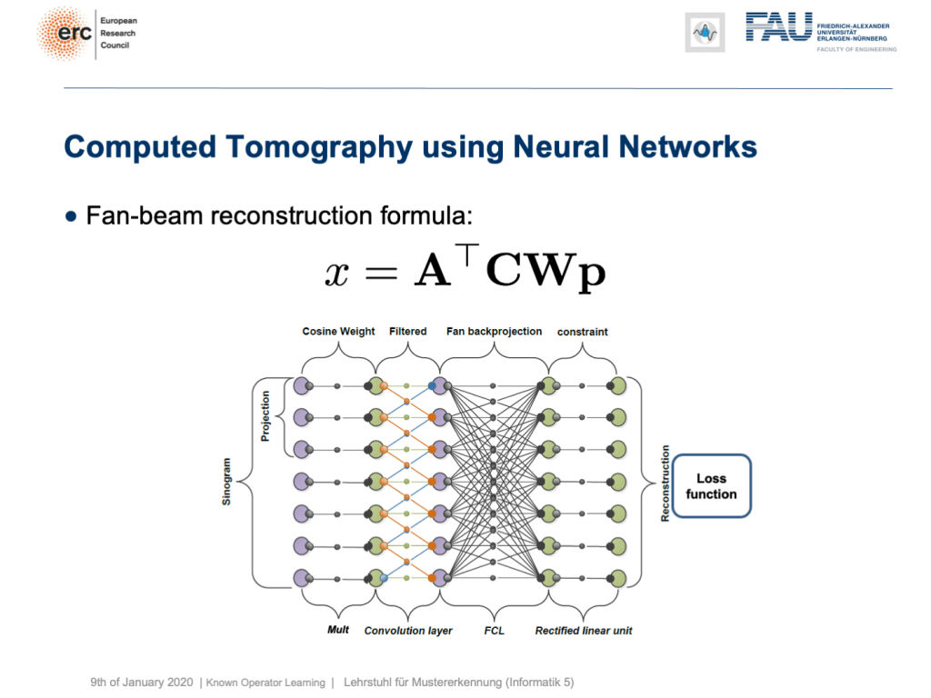
You can see that you can approximate also fan-beam reconstruction with similar matrix kinds of equations. We have now an additional matrix W. So, W is a point-wise weight that is multiplied to each pixel in the input image. C is now directly our convolutional matrix. So, we can describe a fan-beam reconstruction formula simply with this equation and of course, we can produce a resulting network out of this.
您会看到,您也可以使用类似矩阵类型的方程来近似扇形束重构。 现在,我们有一个附加矩阵W。 因此, W是逐点权重,它乘以输入图像中的每个像素。 C现在直接是我们的卷积矩阵。 因此,我们可以简单地用该方程式来描述扇形束重建公式,当然,我们可以由此产生一个结果网络。
Now let’s look at what happens if we go back to this limited angle tomography problem. So, if you have a complete scan, it looks like this. Let’s go to a scan that has only 180 degrees of rotation. Here, the minimal set for the scan would be actually 200 degrees. So, we are missing 20 degrees of rotation. Not as strong as the limited angle problem that I showed in the introduction of known operator learning, but still significant artifact emerges here. Now, let’s take as pre-training our traditional filtered back-projection algorithm and adjust the weights and the convolution. If you do so, you get this reconstruction. So, you can see that the image quality is dramatically improved. A lot of the artifact is gone. There are still some artifacts on the right-hand side, but image quality is dramatically better. Now, you could argue “Well, you are again using a black box!”.
现在让我们看一下如果回到这个有限角度层析成像问题 。 因此,如果您有完整的扫描,则看起来像这样。 让我们转到只有180度旋转的扫描。 在这里,扫描的最小集实际上是200度。 因此,我们缺少20度旋转。 虽然不如我在介绍已知的操作员学习中所介绍的有限角度问题那么强,但这里仍然出现了明显的工件。 现在,让我们对传统的滤波反投影算法进行预训练,并调整权重和卷积。 如果这样做,您将获得此重建。 因此,您可以看到图像质量得到了显着改善。 许多工件消失了。 右侧仍然有一些伪像,但是图像质量明显更好。 现在,您可以争论“嗯,您又在使用黑匣子!”。
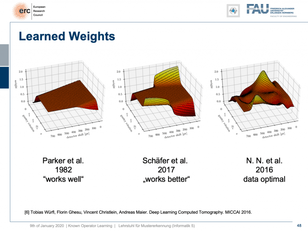
but that’s not actually true because our weights can be mapped back into the original interpretation. We still have a filtered back-projection algorithm. This means we can read out the trained weights from our network and compare them to the state-of-the-art. If you look here, we initialized with the so-called Parker weights which are the solution to a short scan. The idea here is that opposing rays are assigned a weight such that the rays that measure exactly the same line integrals essentially sum up to one. This is shown on the left-hand side. On the right-hand side, you find the solution that our neural network found in 2016. So this is the data-optimal solution. You see it did significant changes to our Parker weights. Now, in 2017 Schäfer et al. published a heuristic how to fix these limited angle artifacts. They suggested ramping up the weight of rays that run through the area where we are missing observations. They simply increase the weight in order to fix the deterministic mass loss. What they found looks better, but is a heuristic. We can see that our neural network found a very similar solution and we can demonstrate that this is data-optimal. So, you can see a distinct difference on the very left and the very light right. If you look here and if you look here, you can see that in these weights, this goes all the way up here and here. This is actually the end of the detector. So, here and here is the boundary of the detector, also here and here. This means we didn’t have any change in these areas here and these areas here. The reason for that is we never had an object in the training data that would fill the entire detector. Hence, we can also not backpropagate gradients here. This is why we essentially have the original initialization still at these positions. That’s pretty cool. That’s really interpreting networks. That’s really understanding what’s happening in the training process, right?
但这并不是真的,因为我们的权重可以映射回原始解释。 我们仍然有一个过滤的反投影算法。 这意味着我们可以从网络中读取经过训练的权重,并将其与最新技术进行比较。 如果您在这里查看,我们将使用所谓的Parker权重进行初始化,这是短期扫描的解决方案。 这里的想法是为相对的光线分配权重,以使测量完全相同的线积分的光线本质上合计为一个。 这显示在左侧。 在右侧,您可以找到我们的神经网络在2016年找到的解决方案。因此,这是数据最优的解决方案。 您会看到它对我们的Parker重量产生了重大变化。 现在,在2017年,Schäfer等人。 发表了启发式的方法来修复这些有限角度的伪影。 他们建议加大穿过我们缺少观测区域的光线的权重。 他们只是增加重量以解决确定性的质量损失。 他们发现的内容看起来更好,但是很启发。 我们可以看到我们的神经网络找到了一个非常相似的解决方案,并且可以证明这是数据最优的。 因此,您可以在最左侧和最右侧看到明显的差异。 如果您看这里,如果您看这里,您会发现这些权重一直都在这里和这里。 这实际上是检测器的结尾。 因此,这里和这里是检测器的边界,也在这里和这里。 这意味着我们在这里和这些区域都没有任何变化。 这样做的原因是我们在训练数据中从来没有一个对象可以填满整个检测器。 因此,我们也不能在此处反向传播梯度。 这就是为什么我们本质上仍将原始初始化保留在这些位置的原因。 太酷了。 那真的是在解释网络。 那真的是了解培训过程中发生的事情,对吗?
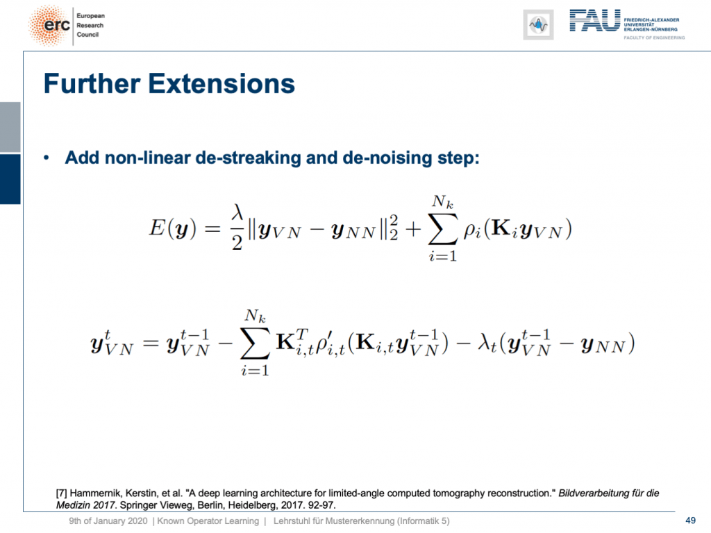
So, can we do more? Yes, there are even other things like so-called variational networks. This is work by Kobler, Pock, and Hammernik and they essentially showed that any kind of energy minimization can be mapped into a kind of unrolled, feed-forward problem. So, essentially an energy minimization can be solved by gradient descent. So, you essentially end up with an optimization problem that you seek to minimize. If you want to do that efficiently, you could essentially formulate this as a recurrent neural network. How did we deal with recurrent neural networks? Well, we unroll them. So any kind of energy minimization can be mapped into a feed-forward neural network, if you fix the number of iterations. This way, you can then take an energy minimization like this iterative reconstruction formula here or iterative denoising formula here and compute its gradient. If you do so, you will essentially end up with the previous image configuration minus the negative gradient direction. You do that and repeat this step by step.
那么,我们还能做更多吗? 是的,甚至还有其他一些东西,例如所谓的变分网络。 这是Kobler,Pock和Hammernik的工作,他们实质上表明,任何一种能量最小化都可以映射为一种展开的前馈问题。 因此,基本上可以通过梯度下降来解决能量最小化问题。 因此,您最终会遇到要最小化的优化问题。 如果您想高效地做到这一点,则可以从本质上将其表述为递归神经网络。 我们如何处理递归神经网络? 好吧,我们将它们展开。 因此,如果您固定迭代次数,则任何形式的能量最小化都可以映射到前馈神经网络。 这样,您就可以像此处的迭代重建公式或此处的迭代去噪公式那样进行能量最小化,并计算其梯度。 如果这样做,您将最终得到先前的图像配置减去负梯度方向。 您这样做,然后逐步重复此步骤。
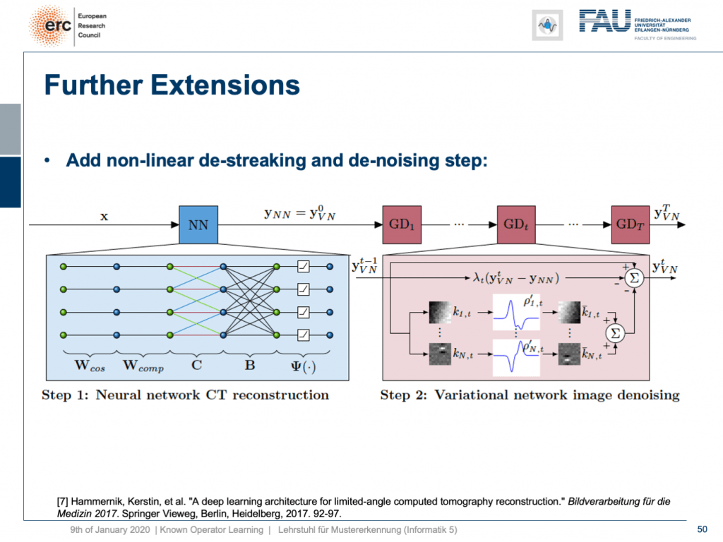
Here, we have a special solution because we combine it with our neural network reconstruction. We just want to learn an image enhancement step subsequently. So what we do is we take our neural network reconstruction and then hook up on the previous layers. There are T streaking or denoising steps that are trainable. They use compressed sensing theory. So, if you want to look into more details here, I recommend taking one of our image reconstruction classes. If you look into them you can see that there is this idea of compressing the image in a sparse domain. Here, we show that we can actually learn the transform that expresses the image contents in a sparse domain meaning that we can also get this new sparsifying transform and interpret it in a traditional signal processing sense.
在这里,我们有一个特殊的解决方案,因为我们将其与我们的神经网络重建相结合。 我们只想随后学习图像增强步骤。 因此,我们要做的是我们进行神经网络重建,然后连接到先前的层。 可以进行T条纹或去噪步骤。 他们使用压缩感测理论。 因此,如果您想在此处了解更多详细信息,建议您参加我们的图像重建课程之一 。 如果查看它们,您会发现存在在稀疏域中压缩图像的想法。 在这里,我们表明,我们实际上可以学习在稀疏域中表示图像内容的变换,这意味着我们也可以获取此新的稀疏变换并以传统的信号处理意义进行解释。
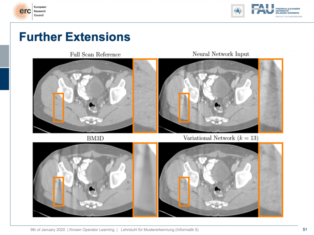
Let’s look at some results. Here, you can see that if we take the full scan reference, we get really an artifact-free image. Our neural network output with this reconstruction network that I showed earlier kind of is improved, but it still has these streak artifacts that you see on the top right. On the bottom left, you see the output of a denoising algorithm that is 3-D. So, this does denoising, but it still has problems with streaks. You can see that in our variational Network on the bottom right, the streaks are quite a bit suppressed. So, we really learn a transform based on the ideas of compressed sensing in order to remove those streaks. A very nice neural network that mathematically exactly models a compressed sensing reconstruction approach. So that’s exciting!
让我们看一些结果。 在这里,您可以看到,如果我们使用完整的扫描参考,则实际上可以获得无伪像的图像。 我之前展示过的带有该重构网络的神经网络输出得到了改进,但是它仍然具有您在右上角看到的这些条纹痕迹。 在左下方,您会看到3-D去噪算法的输出。 因此,这确实是去噪的,但是仍然存在条纹问题。 您可以看到在右下角的变化网络中,条纹受到了很大的抑制。 因此,我们确实学习了基于压缩感测思想的变换,以消除这些条纹。 一个非常不错的神经网络,可以在数学上精确地模拟压缩感测重建方法。 真令人兴奋!
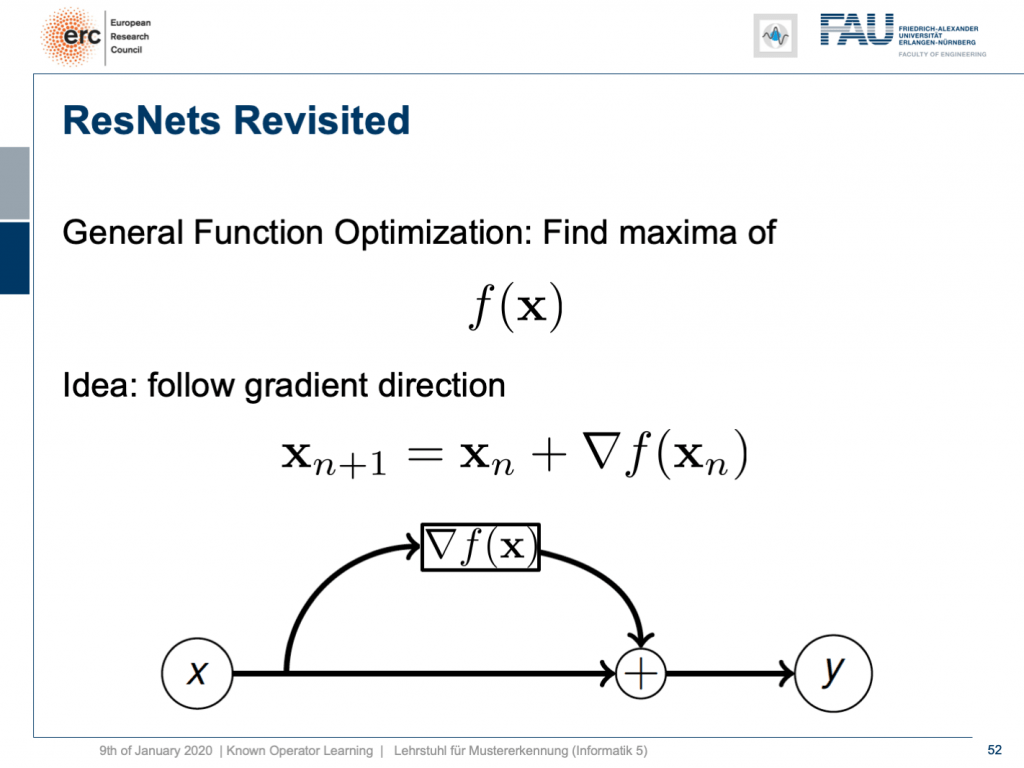
By the way, if you think of this energy minimization idea, then you also find the following interpretation: The energy minimization and this unrolling always lead to a ResNet because you take the previous configuration minus the negative gradient direction meaning that it’s the previous layers output plus the new layer’s configuration. So, this essentially means that ResNets can also be expressed in this kind of way. They always are the result of any kind of energy minimization problem. It could also be a maximization. In any case, we don’t even have to know whether it’s a maximization or minimization, but generally, if you have a function optimization, then you can always find the solution to this optimization process through a ResNet. So, you could argue that ResNets are also suited to find the optimization strategy for a completely unknown error function.
顺便说一句,如果您想到这种能量最小化的想法,那么您还会发现以下解释:能量最小化和这种展开始终会导致ResNet,因为您采用了先前的配置减去负梯度方向,这意味着它是先前的层输出加上新层的配置。 因此,这实质上意味着ResNets也可以以这种方式表示。 它们始终是任何形式的能量最小化问题的结果。 这也可能是一个最大化。 无论如何,我们甚至都不必知道这是最大化还是最小化,但是通常,如果您进行了功能优化,则始终可以通过ResNet找到该优化过程的解决方案。 因此,您可能会说ResNets也适合为完全未知的误差函数找到优化策略。
Interesting, isn’t it? Well, there are a couple of more things that I want to tell you about these ideas of known operator learning. Also, we want to see more applications where we can apply this and maybe also some ideas on how the field of deep learning and machine learning will evolve over the next couple of months and years. So, thank you very much for listening and see you in the next and final video. Bye-bye!
有趣,不是吗? 好吧,关于这些关于已知操作员学习的想法,我想告诉您更多其他内容。 此外,我们希望看到更多可以在其中应用的应用程序,并且可能还需要一些关于深度学习和机器学习领域在未来几个月和几年中将如何发展的想法。 因此,非常感谢您的收听,并在下一个也是最后一个视频中见到您。 再见!
If you liked this post, you can find more essays here, more educational material on Machine Learning here, or have a look at our Deep LearningLecture. I would also appreciate a follow on YouTube, Twitter, Facebook, or LinkedIn in case you want to be informed about more essays, videos, and research in the future. This article is released under the Creative Commons 4.0 Attribution License and can be reprinted and modified if referenced. If you are interested in generating transcripts from video lectures try AutoBlog.
如果你喜欢这篇文章,你可以找到这里更多的文章 ,更多的教育材料,机器学习在这里 ,或看看我们的深入 学习 讲座 。 如果您希望将来了解更多文章,视频和研究信息,也欢迎关注YouTube , Twitter , Facebook或LinkedIn 。 本文是根据知识共享4.0署名许可发布的 ,如果引用,可以重新打印和修改。 如果您对从视频讲座中生成成绩单感兴趣,请尝试使用AutoBlog 。
谢谢 (Thanks)
Many thanks to Weilin Fu, Florin Ghesu, Yixing Huang Christopher Syben, Marc Aubreville, and Tobias Würfl for their support in creating these slides.
非常感谢傅伟林,弗洛林·格苏,黄宜兴Christopher Syben,马克·奥布雷维尔和托比亚斯·伍尔夫(TobiasWürfl)为创建这些幻灯片提供的支持。
翻译自: https://towardsdatascience.com/known-operator-learning-part-3-984f136e88a6
已知两点坐标拾取怎么操作


 1万+
1万+

 被折叠的 条评论
为什么被折叠?
被折叠的 条评论
为什么被折叠?
 到【灌水乐园】发言


