


已知两点坐标拾取怎么操作
有关深层学习的FAU讲义 (FAU LECTURE NOTES ON DEEP LEARNING)
These are the lecture notes for FAU’s YouTube Lecture “Deep Learning”. This is a full transcript of the lecture video & matching slides. We hope, you enjoy this as much as the videos. Of course, this transcript was created with deep learning techniques largely automatically and only minor manual modifications were performed. Try it yourself! If you spot mistakes, please let us know!
这些是FAU YouTube讲座“ 深度学习 ”的 讲义 。 这是演讲视频和匹配幻灯片的完整记录。 我们希望您喜欢这些视频。 当然,此成绩单是使用深度学习技术自动创建的,并且仅进行了较小的手动修改。 自己尝试! 如果发现错误,请告诉我们!
导航 (Navigation)
Previous Lecture / Watch this Video / Top Level / Next Lecture
Welcome back to deep learning! So, today I want to continue to talk to you about known operators. In particular, I want to show you how to embed these known operations into the network and what kind of theoretical implications are created by this. So, the key phrase will be “Let’s not re-invent the wheel.”
欢迎回到深度学习! 因此,今天我想继续与您谈谈已知的运营商。 特别是,我想向您展示如何将这些已知的操作嵌入到网络中,以及由此产生的理论意义。 因此,关键词将是“让我们不要重新发明轮子”。

We go back all the way to our universal approximation theorem. The universal approximation theorem told us that we can find a one hidden layer representation that approximates any continuous function u(x) with an approximation U(x) and it is supposed to be very close. It’s computed as a superposition linear combination of sigmoid functions. We know that there is a bound ε subscript u. ε subscript u tells us the maximum difference between the original function and the approximated function and this is exactly one hidden layer in your network.
我们一直回到通用逼近定理 。 通用逼近定理告诉我们,我们可以找到一个隐层表示,它以近似值U( x )近似任何连续函数u( x ),并且应该非常接近。 它作为S型函数的叠加线性组合进行计算。 我们知道存在一个有界的ε下标u。 ε下标u告诉我们原始函数和近似函数之间的最大差值,而这恰恰是网络中的一个隐藏层。

Well, this is nice but we are not really interested in one-hidden-layer neural networks, right? We would be interested in an approach that we coined precision learning. So here, the idea is that we want to mix approximators with known operations and embed them into the network. Specifically, the configuration that I have here is a little big for theoretical analysis. So, let’s go to a little simpler problem. Here, we just say okay we have a two-layer network where we have a transform from xusing u(x). So, this is a vector to vector transform. This is why it’s in boldface. Then, we have some transform g(x). It takes the output of u(x) and produces a scalar value. This is then essentially the definition of f(x). So here, we know that f(x) is composed of two different functions. So, this is already the first postulate here that we need in order to look into known operator learning.
好吧,这很好,但是我们对单层神经网络并不真正感兴趣,对吗? 我们会对我们创造精确学习的方法感兴趣。 因此,这里的想法是,我们希望将逼近器与已知运算混合,并将其嵌入网络中。 具体来说,这里的配置对于理论分析来说有点大。 因此,让我们处理一个简单的问题。 在这里,我们只是说好,我们有一个两层网络,其中我们使用u ( x )从x进行了转换。 因此,这是向量到向量的转换。 这就是为什么它以粗体显示。 然后,我们有一些变换g( x )。 它获取u ( x )的输出并产生标量值。 因此,这实质上是f( x )的定义。 因此,在这里,我们知道f( x )由两个不同的函数组成。 因此,这已经是我们研究已知的操作员学习所需的第一个假设。

We now want to approximate composite functions. If I look at f, we can see that there are essentially three choices of how we can approximate it. We can approximate only U(x). Then, this would give us F subscript u. We could approximate only G(x). This would result in F subscript g, or we could approximate both of them. That is then G(U(x)) using both of our approximations. Now, with any of these approximations, I’m introducing an error. The error can be described as e subscript u, if I approximate U(x) and e subscript g, if I approximate G(x), and e subscript f, if I approximate both.
现在,我们要近似复合函数。 如果我看f,我们可以看到在如何近似上有三种选择。 我们只能近似U ( x )。 然后,这将给我们F下标u。 我们只能近似G( x )。 这将导致F下标g,或者我们可以将两者近似。 那么,使用我们的两个近似值就是G( U ( x ))。 现在,使用任何这些近似值,我都会引入一个错误。 如果我近似于U ( x ),则误差可描述为e下标u;如果我近似于G( x ),则误差可描述为e下标;如果我近似于两者,则误差可描述为e下标f。

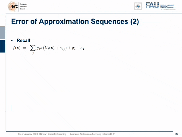
So, let’s look into the math and see what we can do with those definitions. Well, of course, we can start with f(x). We use the definition of f(x). Then, the definition gives us g(u(x)). We can start approximating G(x). Now, if you’re approximate it, we introduce some error e subscript g. The error has to be added back. This is then shown here in the next line. We can see we can also use the definition of G(x) that is a linear combination of sigmoid functions. Here, we then use component-wise the original function u subscript j, because it is a vectorial function. Of course, we have the different weights g subscript j, the bias g subscript 0, and the error that we introduced by approximating g(x). So, we can also now approximate u(x) component-wise. Then, we introduce an approximation and the approximation, of course, also introduces an error. So, this is nice, but we kind of get stuck here because the error of the approximation of u(x) is inside of the sigmoid function. All the other errors are outside. So, what can we do about this? Well, least we can look into error bounds.
因此,让我们看一下数学,看看我们可以用这些定义做什么。 好吧,当然,我们可以从f( x )开始。 我们使用f( x )的定义。 然后,定义给出g( u ( x ))。 我们可以开始近似G( x )。 现在,如果您大致估计一下,我们将介绍一些误差e下标g。 该错误必须重新添加。 然后在下一行中显示。 我们可以看到我们也可以使用G( x )的定义,它是S型函数的线性组合。 在这里,我们然后按分量使用原始函数u下标j,因为它是矢量函数。 当然,我们有不同的权重g下标j,偏差g下标0和近似g( x )引入的误差。 因此,我们现在也可以逐分量地近似u ( x )。 然后,我们介绍一个近似值,当然,这个近似值也引入一个误差。 因此,这很好,但是我们有点卡在这里,因为u ( x )的近似误差在S型函数内。 所有其他错误不在外面。 那么,我们该怎么办? 好吧,至少我们可以研究误差范围。

So, let’s have a look at our bounds. The key idea here is that we use the property of the sigmoid function that it has a Lipschitz bound. So, there is a maximum slope that occurs in this function and that is denoted by l subscript s meaning that if I’m at the position x and I move to a direction e, then I can always find an upper bound by taking the magnitude of e times the highest slope that occurs in the function plus the original function value. So, it’s a linear extrapolation and you can see this in this animation. We essentially have the two white cones that always will be above or below the function. Obviously, we can also construct a lower bound using the Lipschitz property. Well, now what can we do with this? We can now go ahead and use it for our purposes but we just run into the next problem. Our Lipschitz bound here doesn’t hold for linear combinations. So, you see that we are actually interested in multiplying this with some weight g subscript j. As soon as I take a negative g subscript j, then this would essentially mean that our inequality flips. So, this is not cool but we can find an alternative formulation like the bottom one. So, we simply have to use an absolute value when we multiply with the Lipschitz constant in order to remain above the function all the time. Running through the proof here is kind of tedious. This is why I brought you the two images here. So, we reformulated this and we took all the terms on the right-hand side, subtracted them, and move them to the left-hand side which means that all of these terms need to be in combination lower than zero. If you do that for positive and negative g subscript j, you can see in the two plots that independent of the choice of e and x, I’m always below zero. You can also go to the original reference if you’re interested in the formal proof for this [5].
因此,让我们来看看我们的界限。 这里的关键思想是我们使用Sigmoid函数的一个具有Lipschitz界的属性。 因此,此函数中存在一个最大斜率,用l下标s表示,这意味着如果我在x位置并且我向e方向移动,那么我总是可以通过取幅值来找到上限e乘以函数中出现的最高斜率加上原始函数值。 因此,这是线性外推,您可以在此动画中看到这一点。 本质上,我们有两个始终位于功能上方或下方的白色圆锥体。 显然,我们还可以使用Lipschitz属性构造一个下限。 好吧,现在我们该怎么办? 我们现在可以继续将其用于我们的目的,但我们遇到了下一个问题。 我们在此处的Lipschitz界限不适用于线性组合。 因此,您看到我们实际上对将其乘以权重g下标j感兴趣。 一旦我给负g下标j,那么这实质上意味着我们的不平等现象开始恶化。 因此,这并不酷,但是我们可以找到另一种替代方法,例如底部的方法。 因此,当我们与Lipschitz常数相乘时,我们仅需使用绝对值即可始终保持在函数上方。 在这里遍历证明有点乏味。 这就是为什么我在这里为您带来了两张图片。 因此,我们对此进行了重新格式化,并在右侧取了所有项,将它们相减,然后将它们移到左侧,这意味着所有这些项的组合都必须小于零。 如果对正负g下标j执行此操作,则可以在两个图中独立于e和x的选择看出,我始终低于零。 如果您对此的正式证明感兴趣,也可以转到原始参考文献[5]。
So now, let’s use this inequality. We can see now that we can finally get our e subscript uj out of the bracket snd out of the sigmoid function. We get an upper bound by using this kind of approximation. Then, we can see if we arrange the terms correctly that the first couple of terms are simply the definition of F(x). So, this is the approximation using G(x) and U(x). This then can be simplified to just write down F(x). This, plus the sum over the components of G(x) times the Lipschitz times the absolute value of the error plus the error that we introduced by G. Now, we can essentially subtract F(x) and if we do so, we can see that f(x) — F(x) is nothing else than the error introduced when doing this approximation. So, this is simply e subscript f. So, we have an upper bound for the error in e subscript f that is composed as the sum on the right-hand side. We can still replace the e subscript g by ε subscript g which is the upper bound to e subscript g. It’s still an upper bound to e subscript f. Now, these are all upper bounds.
现在,让我们使用这个不等式。 现在我们可以看到,我们终于可以从S型函数的括号snd中获得e下标uj。 通过使用这种近似,我们得到了一个上限。 然后,我们可以看到我们是否正确安排了这些术语,即前几对术语仅仅是F( x )的定义。 因此,这是使用G( x )和U ( x )的近似值。 然后可以简化为仅记下F( x )。 加上G( x )的总和乘以Lipschitz乘以误差的绝对值再加上G引入的误差。现在,我们基本上可以减去F( x ),如果这样做,我们可以看到f( x )— F( x )就是进行这种近似时引入的误差。 因此,这仅仅是e下标f。 因此,我们有一个e下标f中的误差的上限,该误差由右边的和组成。 我们仍然可以用e下标g的上限ε下标g替换e下标g。 它仍然是e下标f的上限。 现在,这些都是上限。

The same idea can also be used to get a lower bound. You see that then we have this negative sum. This is always a lower bound. Now, if we have the upper and the lower bound, then we can see that the magnitude of e subscript f is bound by the sum over the components g subscript j times the Lipschitz constant times the error plus ε subscript g. This is interesting because here we see that this is essentially the error of U(x) amplified with the structure of G(x) plus the error introduced by G. So, if we know u(x) the error u cancels out, and if we know g(x) the error g cancels out, and of course, if we know both, there is no error because there’s nothing that we have to learn.
同样的想法也可以用来获得下界。 您看到,那么我们有这个负数。 这始终是一个下限。 现在,如果我们有上限和下限,那么我们可以看到e下标f的大小由分量g下标j的和乘Lipschitz常数乘以误差加ε下标g的总和来约束。 这很有趣,因为在这里我们看到这本质上是U ( x )的误差被G( x )结构放大,再加上G引入的误差。因此,如果我们知道u ( x ),则误差u被抵消,如果我们知道g( x ),那么错误g就会抵消,当然,如果我们都知道,就不会有错误,因为我们不需要学习任何东西。

So, we can see that this bound has these very nice properties. If we now relate this to classical pattern recognition, then we could interpret u(x) as a feature extractor and g(x) as a classifier. So, you see that if we do errors in u(x), they get potentially amplified by g(x). This also gives us hints why in classical pattern recognition there was this very high focus on feature extraction. Any feature that you don’t extract correctly, is simply missing. This is also a big advantage of our deep learning approaches. We can also optimize the feature extraction with respect to the classification. Note that when deriving all of this we required Lipschitz continuity.
因此,我们可以看到此绑定具有这些非常好的属性。 如果现在将其与经典模式识别相关联,则可以将u ( x )解释为特征提取器,将g( x )解释为分类器。 因此,您会看到,如果我们对u ( x )进行错误处理,则它们有可能被g( x )放大。 这也为我们提供了暗示,为什么在经典模式识别中会如此高度关注特征提取。 您未正确提取的任何功能都将丢失。 这也是我们深度学习方法的一大优势。 我们还可以针对分类优化特征提取。 请注意,在得出所有这些结果时,我们需要Lipschitz连续性。

Okay. Now, you may say “This is only for two layers!”. We also extended this for deep networks. So, you can actually do this. Once you have the two-layer constellation, you can find a proof by recursion that there’s also a bound for deep networks. Then, you essentially get a sum over the layers to find this upper bound. It still holds that it’s the error that is introduced by the respective layer that contributes in an additive way to the total error bound. Again, if I know one layer that part of the error is gone, and the total upper bound is reduced nicely. We managed to publish this in nature machine intelligence. So, seemingly this was an interesting result also for other researchers. Okay. Now, we talked about the theory of why it makes sense to include known operations into deep networks. So, it’s not just common sense knowledge that we want to reuse these priors, but we can actually formally show that we’re reducing the error bounds.
好的。 现在,您可能会说“这仅适用于两层!”。 我们还将其扩展到深层网络。 因此,您实际上可以执行此操作。 一旦有了两层星座,就可以通过递归找到证明深层网络也必不可少的证据。 然后,您实际上可以得到各层的总和以找到该上限。 仍然认为,由各个层引入的误差以累加的方式对总误差范围做出了贡献。 同样,如果我知道一层错误已经消失了,那么总的上限就会很好地降低。 我们设法将其发布在自然界的机器智能中。 因此,看来这对其他研究人员来说也是一个有趣的结果。 好的。 现在,我们讨论了为什么将已知操作包含到深度网络中才有意义的理论。 因此,我们不仅要重用这些先验知识,还可以正式表明我们正在减少错误界限。

So in the next lecture, we want to look into a couple of examples of this. Then, you will also see how many different applications actually use this. So, thank you very much for listening and see you in the next video. Bye-bye!
因此,在下一个讲座中,我们想研究几个示例。 然后,您还将看到实际上有多少个不同的应用程序使用此功能。 因此,非常感谢您的收听,并在下一个视频中与您相见。 再见!
If you liked this post, you can find more essays here, more educational material on Machine Learning here, or have a look at our Deep LearningLecture. I would also appreciate a follow on YouTube, Twitter, Facebook, or LinkedIn in case you want to be informed about more essays, videos, and research in the future. This article is released under the Creative Commons 4.0 Attribution License and can be reprinted and modified if referenced. If you are interested in generating transcripts from video lectures try AutoBlog.
如果你喜欢这篇文章,你可以找到这里更多的文章 ,更多的教育材料,机器学习在这里 ,或看看我们的深入 学习 讲座 。 如果您希望将来了解更多文章,视频和研究信息,也欢迎关注YouTube , Twitter , Facebook或LinkedIn 。 本文是根据知识共享4.0署名许可发布的 ,如果引用,可以重新打印和修改。 如果您对从视频讲座中生成成绩单感兴趣,请尝试使用AutoBlog 。
谢谢 (Thanks)
Many thanks to Weilin Fu, Florin Ghesu, Yixing Huang Christopher Syben, Marc Aubreville, and Tobias Würfl for their support in creating these slides.
非常感谢傅伟林,弗洛林·格苏,黄宜兴Christopher Syben,马克·奥布雷维尔和托比亚斯·伍尔夫(TobiasWürfl)为创建这些幻灯片提供的支持。
翻译自: https://towardsdatascience.com/known-operator-learning-part-2-8c725b5764ec
已知两点坐标拾取怎么操作


 209
209


 被折叠的 条评论
为什么被折叠?
被折叠的 条评论
为什么被折叠?
 到【灌水乐园】发言


