pagerank_pagerank的手写介绍

pagerank

Google owes a great part of its success to the algorithm which was originally used to rank webpages. This algorithm, PageRank, sorts all the pages of a network according to their popularity. The more webpages link to some page A, the highest its score is and the most likely it is to appear among the top results of a search. The example of PageRank is commonly given in linear algebra courses, as it is a good illustration of the applications of eigenvalues and eigenvectors. This article aims at building an intuitive understanding of PageRank and will show the maths and the code behind it.

Google的成功很大程度上归功于最初用于对网页进行排名的算法。 PageRank这个算法根据网络的受欢迎程度对网络中的所有页面进行排序。 链接到某个页面A的网页越多，其得分最高，并且最有可能出现在搜索结果的顶部。 PageRank的示例通常在线性代数课程中给出，因为它很好地说明了特征值和特征向量的应用。 本文旨在建立对PageRank的直观了解，并展示其背后的数学和代码。

It assumes basic knowledge of linear algebra, including manipulating matrices and vectors. Prior knowledge of eigenvalues and eigenvectors will be helpful, albeit not indispensable. We will illustrate the algorithm with a pure implementation in Python and Numpy as well as with the library NetworkX.

它假定了线性代数的基本知识，包括操纵矩阵和向量。 特征值和特征向量的先验知识将是有帮助的，尽管不是必不可少的。 我们将使用Python和Numpy以及库NetworkX的纯实现来说明该算法。

Let’s start by setting up a tiny internet. It consists of six webpages which contain links to other pages or themselves. We can represent this network as an oriented graph, like in the messy drawing below.

让我们从建立一个小型互联网开始。 它由六个网页组成，这些网页包含指向其他页面或自身的链接。 我们可以将该网络表示为有向图，如下面的混乱图所示。

Gamma.

伽玛

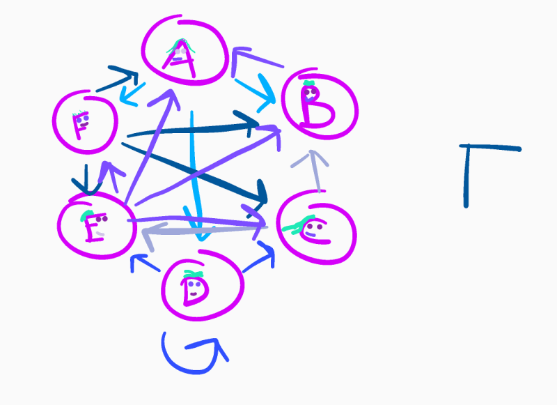
We will represent this graph with an adjacency matrix where the value at row r and column c is the probability of landing on the webpage r given that you have just followed a link from the webpage c. For example, page A links to pages B, D and F. Since there are three destinations, we normalise our vector by a factor of 1/3, which gives us:

我们将用一个邻接矩阵来表示该图，其中假设您刚刚跟随了网页c的链接，则行r和列c的值是登陆到网页r的概率。 例如，页面A链接到页面B，D和F。由于存在三个目标，因此我们将向量归一化1/3 ，从而得出：

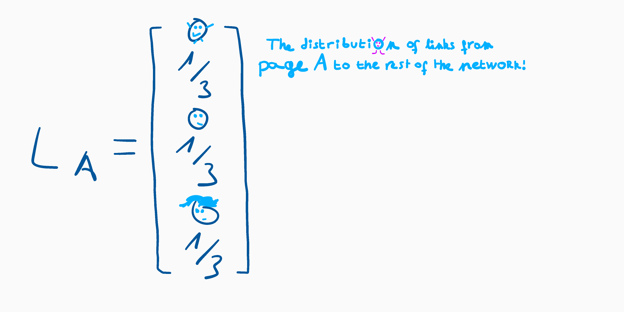
We called this vector L[A], which stands for Link from page A.

我们称此向量L[A] ，它表示A页上的Link 。

By applying the same process to all our pages, we get the link matrix shown below.

通过对所有页面应用相同的过程，我们得到如下所示的链接矩阵。

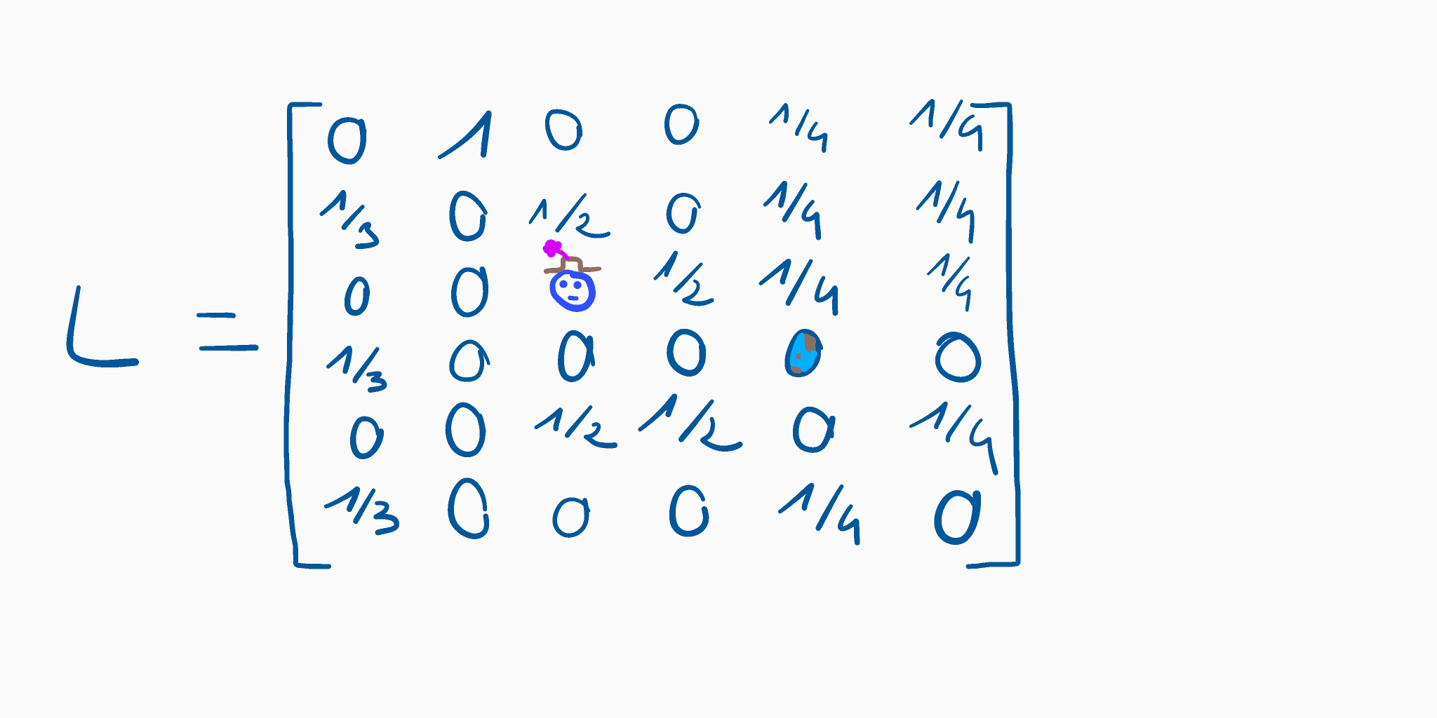
Although you may find implementations that behave differently, our link matrix ignores self-referencing links. We don’t consider multiple references to the same target either.

尽管您可能会发现实现方式有所不同，但是我们的链接矩阵忽略了自引用链接。 我们也不考虑对同一目标的多次引用。

Before jumping into a more abstract description of PageRank, this extract from the original paper published in 1998 (link in the footnotes) can give you a good perception of what the algorithm does:

在进入更抽象的PageRank描述之前，请摘录于1998年发表的原始论文(脚注中的链接)的摘录，可以使您对算法的功能有一个很好的认识：

Intuitively, this can be thought of as modeling the behavior of a “random surfer”. The “random surfer” simply keeps clicking on successive links at random.

直观地，这可以被认为是对“随机冲浪者”的行为进行建模。 “随机浏览者”只是继续随机点击连续的链接。

The idea behind PageRank is to give each page a popularity score, which we call a rank. If the surfers often land on some webpage, it means that many other pages recommend it, and, therefore, that it may be good. The goal of the algorithm is to find the probability that the random surfers end up on each page as they stroll around the internet.

PageRank背后的想法是给每个页面一个受欢迎程度得分，我们将其称为rank 。 如果冲浪者经常登陆某个网页，则意味着许多其他网页都推荐它，因此，它可能是不错的选择。 该算法的目的是发现随机冲浪者在互联网上漫步时最终出现在每个页面上的可能性。

The n-th row of the matrix indicates all the pages that contain a reference to the n-th page and the probability of reaching it. By summing all the values on each row, we could determine a first popularity score. But we also need to consider the popularity of the page which contains the reference, as you’d better be mentioned by a popular page than one which is rarely visited. We can translate this description into an iterative formula where the popularity of the page A depends on each reference that links to it, weighted by the popularity of the page that contains the reference:

矩阵的第n行指示包含对第n页的引用及其到达概率的所有页。 通过将每一行上的所有值相加，我们可以确定第一受欢迎度得分。 但是，我们还需要考虑包含参考的页面的受欢迎程度，因为与不常访问的页面相比，最好在受欢迎的页面中提及您。 我们可以将此描述转换为一个迭代公式，其中页面A的受欢迎程度取决于链接到它的每个引用，并通过包含该引用的页面的受欢迎程度进行加权：

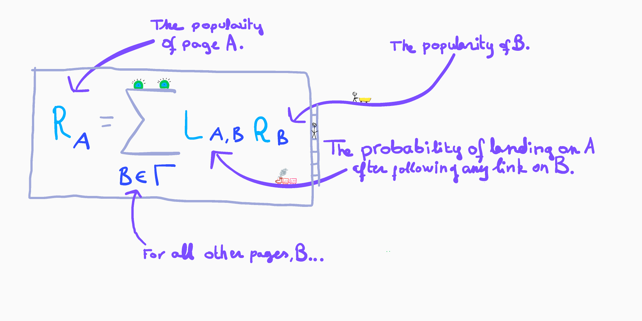
We can generalise and simplify the expression above by writing it as the product of the link matrix L by a column matrix R which contains the popularity score of each webpage:

我们可以通过将其表达为链接矩阵L与包含每个网页的受欢迎程度得分的列矩阵R的乘积，来概括和简化上面的表达式：

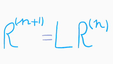
We evaluate this expression until it converges, i.e. until the popularity of all webpages does not change when multiplied to the link matrix. In other words, this operation boils down to finding the eigenvectors of eigenvalue 1 of the link matrix. Given the size of the matrix — which can quickly become extremely large— using this recursive formula, known as the power method, is one of the most efficient ways of solving the problem.

我们评估该表达式，直到收敛为止，即，直到所有网页的受欢迎程度在与链接矩阵相乘时都不变。 换句话说，该操作归结为找到链接矩阵的特征值1的特征向量。 给定矩阵的大小(可能很快变得非常大)，使用这种称为幂方法的递归公式是解决问题的最有效方法之一。

Let’s take a look at a simple implementation in Python:

让我们看一下Python中的一个简单实现：

def rank_websites(links: np.ndarray, threshold: float = 1e-4):
    size = links.shape[0]
    initial = np.ones(size) * 1/size
    previous_ranking: np.ndarray = initial
    iterations = 1
    popularity = links @ initial

    while np.linalg.norm(previous_ranking - popularity) > threshold:        previous_ranking = popularity
        popularity = links @ popularity        iterations += 1

    return popularity, iterations

The function takes in two parameters: the link matrix as a Numpy array and a threshold, set to 1×10^{-4} by default. The threshold corresponds to the tolerance when checking if the popularity has converged.

该函数接受两个参数：作为Numpy数组的链接矩阵和阈值，默认情况下设置为1×10 ^ {-4}。 该阈值对应于检查人气是否收敛时的容差。

We start by creating our initial popularity vector, where the popularity of each page is uniformly distributed.

我们首先创建初始的流行度向量，其中每个页面的流行度均匀分布。

We also need to store the previous popularity vector, which we will use to check if it has converged.

我们还需要存储以前的流行度向量，我们将使用它来检查其是否收敛。

We can now iterate while the norm of the difference between the previous and the current ranking vector is greater than the threshold.

现在，我们可以进行迭代，而前一个和当前排名向量之间的差的范数大于阈值。

If we evaluate this function with our link matrix L, we get the following output (I multiplied it by 100 to make it more legible) after 35 iterations:

如果使用链接矩阵L评估此函数，则经过35次迭代后，我们得到以下输出(我将其乘以100以使其更清晰)：

[29.12342755 22.33189164 11.64928625 9.71001964 13.98001348 13.20536144]

Keep in mind that our method only gives an approximation of the eigenvectors of eigenvalue 1 of the link matrix. Since the network is small enough, we can compare our results with the ones returned by the eigenvector calculator of Numpy:

请记住，我们的方法仅给出链接矩阵特征值1的特征向量的近似值。 由于网络足够小，我们可以将结果与Numpy的特征向量计算器返回的结果进行比较：

eigenvalues, eigenvectors = np.linalg.eig(L)
order = np.absolute(eigenvalues).argsort()[::-1]
eigenvectors = eigenvectors[:, order]
r = eigenvectors[:, 0]
normalised_r = r / np.sum(r)print("using numpy eig function, r =", 100 * normalised_r)

This code starts by fetching the eigenvalues and eigenvectors of the link matrix. We then compute the order of the indices based on their eigenvalue in line 2), which we use to sort the eigenvectors by increasing eigenvalue (in line 3). We extract the eigenvector with the highest eigenvalue in line 4, which we normalise to make it stochastic. This gives us the following result:

此代码从获取链接矩阵的特征值和特征向量开始。 然后，我们根据第2行中的特征值来计算索引的顺序，我们将其用于通过增加特征值来对特征向量进行排序(第3行)。 我们在第4行中提取特征值最高的特征向量，然后对其进行归一化以使其随机。 这给我们以下结果：

[29.12621359-0.j 22.33009709-0.j 11.65048544-0.j  9.70873786-0.j
 13.98058252-0.j 13.2038835 -0.j]

阻尼系数 (The Damping Factor)

The previous implementation worked perfectly fine with a simple example. But we don’t expect all networks to be as well-behaved: if we consider more examples and some special cases, we may stumble upon some unexpected results. Let’s take the following graph, Delta, as an example:

前面的实现通过一个简单的示例就可以很好地工作。 但是我们并不期望所有网络都表现良好：如果我们考虑更多示例和一些特殊情况，可能会偶然发现一些意想不到的结果。 让我们以下图Delta为例：

Delta.

三角洲。

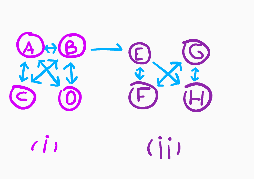
The network is separated into two sub-networks that we called (i) and (ii). (i) and (ii) are connected by a one-way link. Therefore, if the random surfers start their quest in (i), the probability that they end up in (ii) is not zero.

该网络分为两个子网，我们分别称为(i)和(ii) 。 (i)和( ii)通过单向链路连接。 因此，如果随机冲浪者在(i)中开始他们的任务，则他们在(ii)中结束的可能性不为零。

However, once they reach it, they cannot go back to (i). If we build the link matrix and compute its main eigenvector, we get the following results:

但是，一旦达到目标，就无法返回(i) 。 如果我们构建链接矩阵并计算其主要特征向量，则会得到以下结果：

[-3.58205484e-01, 0.00000000e+00, 7.61186653e-01, 2.23878427e-02, 4.06650495e+14, -8.13300990e+14, 1.21995149e+15, -8.13300990e+14]

As we could expect, the pages in (ii) have a much higher rank than those in (i). A common example of such sub-networks is Wikipedia: a lot of pages contain a reference towards it, but Wikipedia pages only contain internal links (external links are “no-follow links”, and therefore are not registered by search engines).

如我们所料， (ii)中的页面比(i)中的页面具有更高的排名。 这种子网的一个常见示例是Wikipedia：很多页面都包含对它的引用，但是Wikipedia页面仅包含内部链接(外部链接是“无关注链接”，因此未由搜索引擎注册)。

The problem of this implementation of PageRank is that it assumes that once you have landed on any page on Wikipedia, you go through all other pages without ever going back or teleporting to another website by typing its URL. Obviously, this approach does not depict the real behaviour of a web surfer and the results it gives are not relevant.

PageRank的此实现的问题在于，它假定一旦您登陆了Wikipedia上的任何页面，便可以浏览所有其他页面，而无需通过键入其URL返回或传送到另一个网站。 显然，这种方法并未描述网络冲浪者的真实行为，并且给出的结果也不相关。

A more conspicuous example of this problem is when the network consists of several graphs which are completely disconnected, like in the example below.

此问题的一个更为明显的示例是当网络由几个完全断开的图形组成时，如以下示例所示。

Epsilon.

Epsilon。

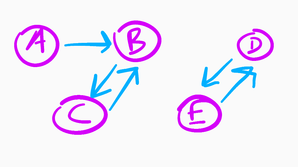
Since there are no relationships between both sub-networks that make up Epsilon, it will be impossible to get a general popularity ranking.

由于组成Epsilon的两个子网之间没有关系，因此不可能获得普遍的人气排名。

If we try to use our algorithm to compute the PageRank of this network, here is the r vector after each of the 10 first iterations:

如果我们尝试使用我们的算法来计算该网络的PageRank，则这是10个首次迭代中的每个迭代之后的r向量：

Initial [0.2 0.2 0.2 0.2 0.2]
1 [0. 0.2 0.4 0.2 0.2]2 [0. 0.4 0.2 0.2 0.2]3 [0. 0.2 0.4 0.2 0.2]4 [0. 0.4 0.2 0.2 0.2]5 [0. 0.2 0.4 0.2 0.2]6 [0. 0.4 0.2 0.2 0.2]7 [0. 0.2 0.4 0.2 0.2]8 [0. 0.4 0.2 0.2 0.2]9 [0. 0.2 0.4 0.2 0.2]10 [0. 0.4 0.2 0.2 0.2]

The rank of pages B and C oscillates between 0.2 and 0.4 without settling. When letting it run a bit longer, it keeps iterating more than 1 million times, without congeriving.

B和C页的等级在0.2到0.4之间波动，而没有稳定下来。 当让它运行更长的时间时，它会不断迭代超过一百万次，而不会引起混乱。

We will use Numpy eigenvectors calculator to try to understand the reason behind this behaviour.

我们将使用Numpy特征向量计算器来尝试了解此行为背后的原因。

eigenvalues: [ 1. -1.  1. -1.  0.]
first eigenvector of eigenvalue 1: [0.         0.         0.         0.70710678 0.70710678]
second eigenvector of eigenvalue 1: [0.         0.70710678 0.70710678 0.         0.        ]

The problem of this network is that it contains multiple eigenvectors of eigenvalue 1: the first vector gives the rank of the network {DE} without considering the other one and the second vector gives the rank of the network {ABC}.

该网络的问题在于它包含多个特征值1的特征向量：第一个向量给出了网络{DE}的等级，而没有考虑另一个特征向量，第二个向量给出了网络{ABC}的等级。

These two examples explain why we need to include an additional parameter to our formula: the Damping Factor. It is described as follows in the original paper:

这两个示例说明了为什么我们需要在公式中包括一个附加参数：阻尼因数。 在原始文件中对此进行了如下描述：

[…] if a real Web surfer ever gets into a small loop of web pages, it is unlikely that the surfer will continue in the loop forever. Instead, the surfer will jump to some other page. The additional factor E can be viewed as a way of modeling this behavior: the surfer periodically “gets bored” and jumps to a random page chosen based on the distribution in E.

[…]如果真正的Web冲浪者曾经进入一个小的网页循环，则该冲浪者不可能永远继续循环。 而是，冲浪者将跳至其他页面。 可以将附加因子E视为对此行为进行建模的一种方式：冲浪者会定期“感到无聊”，并跳转到根据E中的分布选择的随机页面。

The damping factor (that we will call d) corresponds to the probability that the random surfer will follow a link in the page they are currently visiting. Therefore, we can view the probability 1 — d as the probability that they type a URL in the search bar and land on a random website.

阻尼因子(我们将其称为d )对应于随机冲浪者遵循其当前正在访问的页面中的链接的概率。 因此，我们可以将概率1 — d视为他们在搜索栏中键入URL并登陆到随机网站的概率。

When using the damping factor, we try to compute the eigenvector of eigenvalue 1 of a new matrix — we will call it L_hat (couldn’t find a way to put a circumflex on a consonant on my keyboard…) — which is an “improved” version of the link matrix L. It is given in terms of d and L by the formula below:

使用阻尼因子时，我们尝试计算新矩阵的特征值1的特征向量-我们将其称为L_hat (找不到在键盘上的辅音上加L_hat音符号的方法……)-这是“改进的”链接矩阵L版本。 通过以下公式根据d和L给出：

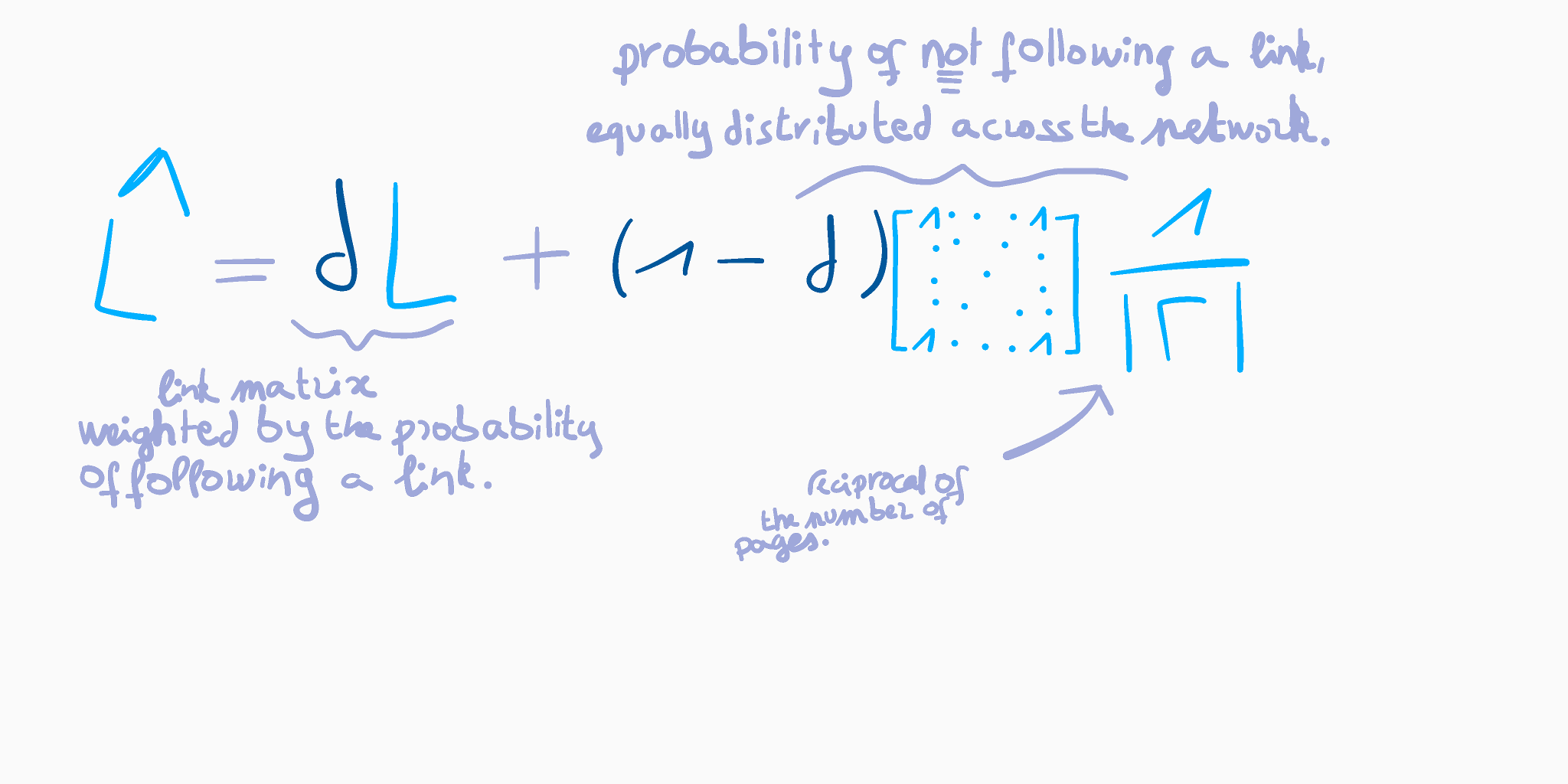
This method helps fixing the problems that we encountered by removing all links with a value of 0.

此方法通过删除所有值为0链接来帮助解决我们遇到的问题。

To update our Python implementation, all we need is to add a new parameter d and write the following line after initialising the size variable:

要更新我们的Python实现，我们所需要做的就是添加一个新参数d并在初始化size变量后编写以下行：

    links = (d * links + (1 - d) * 1/size)

Note the the matrix containing 1‘s everywhere is necessary in the mathematical statement because subtracting a scalar to a matrix is not defined, but this operation is implicit when using Numpy arrays (it will take away the value from each entry of the matrix).

注意包含基质1的无处不在数学陈述必要的，因为减去标量的矩阵没有被定义，但使用numpy的阵列(它会带走从矩阵的每个条目的值)时，该操作是隐式的。

Let’s now test our improved implementation with the graph Delta. Instead of getting huge ranks in the magnitude of 10^{14} for the pages in the second sub-network and minuscule ones orbiting around 10^{-1} for the pages in the first network, we obtain much more realistic results when using a damping factor of 0.85:

现在让我们用图Delta测试改进的实现。 在使用第二个子网中的页面时，与其在第10^{14}个子网中的页面上获得10^{14}巨大排名，而在第一个网络中的页面中绕过10^{-1}左右的微小链接，我们可以获得更现实的结果阻尼系数为0.85 ：

[0.1011186, 0.10702601, 0.07014488, 0.07014488, 0.10941522, 0.15981798, 0.22251445, 0.15981798]

Overall, the sub-network (ii) remains more popular than (i). But all ranks are in the same magnitude, which corroborates the intuition that we would have and prevents pages which contain no outbound links from absorbing all the traffic.

总体而言，子网(ii)仍然比(i)受欢迎。 但是所有级别的级别都相同，这证实了我们的直觉，并阻止了不包含出站链接的页面吸收所有流量。

The damping factor also enables our random surfers to teleport through Epsilon. Therefore, PageRank now yields a consistent distribution across the network:

阻尼因子还使我们的随机冲浪者可以通过Epsilon传送。 因此，PageRank现在可以在整个网络中产生一致的分布：

[0.03 0.2918891 0.2781109 0.2 0.2 ]

Page A has a non-zero rank, even if nobody recommends it ; and all entries add up to 1. This means that they correspond to the probability of landing on each page with respect to the entire network instead of local sub-graphs.

即使没有人推荐，页面A的排名也不为零； 并且所有条目的总和为1。这意味着它们对应于整个网络而不是本地子图在每个页面上着陆的概率。

使用NetworkX (Using NetworkX)

Now that we know how PageRank works, we can simply use its implementation in NetworkX. NetworkX is a Python library that enables to manipulate graphs. Here is how you can do it.

现在我们知道PageRank的工作原理，我们可以简单地在NetworkX中使用其实现。 NetworkX是一个Python库，可用于操作图形。 这是您的操作方法。

1. Installing networkx.

   安装networkx 。

$pip install networkx

2. Building the graph. There are several ways of doing it, one of the most useful one being the function from_numpy_matrix. It takes in a Numpy adjacency matrix (the link matrix) and returns the graph:

2.构建图。 有多种方法可以使用，最有用的方法之一是from_numpy_matrix函数。 它接受一个Numpy邻接矩阵(链接矩阵)并返回图：

import networkx as nxinternet = nx.from_numpy_matrix(L)

3. Computing the page rank. Here again, there exists multiple functions that do the work differently. The two main ones are pagerank, which iterates a given number of times and raises an exception if the network does not converge ; and pagerank_numpy which uses Numpy to calculate the eigenvector of the adjacency matrix of the graph.

3.计算页面等级。 同样，这里存在多个功能不同的功能。 主要的两个是pagerank ，它迭代给定的次数并在网络不收敛的情况下引发异常; 和pagerank_numpy ，它使用Numpy来计算图的邻接矩阵的特征向量。

nx.pagerank(graph, alpha=0.85, max_iter=100)
nx.pagerank_numpy(graph, alpha=0.85)

The example above shows a basic usage of these two functions. The parameter alpha is the damping factor. For more information, here are the links to the documentation of both functions.

上面的示例显示了这两个功能的基本用法。 参数alpha是阻尼系数。 有关更多信息，这是这两个函数的文档的链接。

翻译自: https://medium.com/@alouizakarie/a-handwritten-introduction-to-pagerank-7ed2fedddb0d

pagerank