前端绘制绘制图表_如何轻松地绘制9种专业图表类型

最新推荐文章于 2024-07-30 11:48:07 发布

weixin_26750481

最新推荐文章于 2024-07-30 11:48:07 发布

阅读量886

点赞数

文章标签： python 数据可视化 canvas 可视化 css

原文链接：https://towardsdatascience.com/how-to-draw-9-professional-chart-types-with-zero-effort-c9eee6d2a9cc

版权

本文介绍如何在前端使用canvas和CSS等技术，无需大量努力就能绘制出9种专业级别的图表，包括数据可视化的实用技巧。

摘要由CSDN通过智能技术生成

前端绘制绘制图表

数据可视 (DATA VIZ)

In this article, I share all tricks of the trade how I draw professional charts every day with minimal effort.

在本文中，我分享了所有交易技巧，如何每天以最小的努力绘制专业图表。

Detailed instructions and core source code, so you can replicate the results and amend them as you please.

详细的说明和核心源代码，因此您可以复制结果并根据需要对其进行修改。

You can also test the ready-made example add-in to get started without writing or compiling any code, in 3 simple steps:

您还可以通过3个简单的步骤测试现成的示例外接程序，以开始使用而无需编写或编译任何代码：

1- Download the Excel add-in installer
2- Activate your free account
3- Test the Magic Button

一键式图表 (1-click charts)

Showing your analysis: challenging but crucial.

显示您的分析： 具有挑战性但至关重要。

Tired after all the hard analytical work, results are now clear to you: so why bother? Unfriendly charting tools make you want to cut this step short.

在完成所有艰苦的分析工作之后，您现在已经清楚了结果：那么，为什么要麻烦呢？不友好的图表工具使您希望缩短此步骤。

Charts with 1-click, using the Magic Button of which I share the source code as well as provide a ready-to-use working example, an approach which can be replicated in any tool/software beyond Excel (used for this demo).

一键单击图表，使用“我的魔力”按钮共享源代码，并提供一个现成的工作示例，该方法可以在Excel(此演示中使用)以外的任何工具/软件中复制。

After you will have chosen your chart type and prepared the dataset, this post shows how-to formatting for the 9 main chart types: Line, Pie, Scatter, Bubble, Ladder, Column, Boxplot, Clustered, Bar.

在您选择图表类型并准备了数据集之后，本文将介绍9种主要图表类型的格式：线，饼图，散点图，气泡，阶梯，列，箱形图，聚类，条形图。

1.折线图：演示视频 (1. Line chart: demo video)

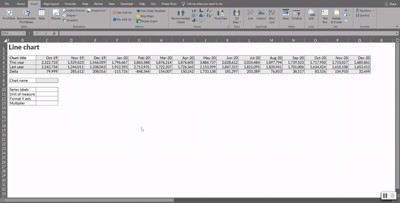
Image for post — Animated demo: the 5 steps of chart creation (CC with attribution)

魔术按钮可在5个简单步骤中缩短图表制作时间 (Magic Button to cut charting short in 5 easy steps)

Step 1. Select the dataset

步骤1.选择数据集

Step 2. Insert regular Excel 2-D line chart then resize it to an approximately 2:1 ratio, which has the best readability

步骤2.插入常规Excel 2-D折线图，然后将其调整为大约2：1的 大小，这具有最佳的可读性

Step 3. Push the Magic button

步骤3.按魔术按钮

Step 4. Set the chart name by looking at the left side of the formula bar, while the chart is selected

步骤4.在选定图表的情况下，通过查看编辑栏的左侧来设置图表名称

Step 5. Fix the 5 finishing touches using appropriate User Defined Functions (UDF)

步骤5.使用适当的用户定义函数(UDF)修复5个修饰点

a. Legend
b. Labels
c. Unit of measure
d. Title
e. Subtitle

绘制用户定义函数(UDF)的图表 (Charting User Defined Functions (UDF))

To achieve full automation even if the data changes, while avoiding some specific bugs of Excel, I use 3 UDF — alternatively, you can implement these finishing touches directly within your Magic Button, but losing some freedom and consistency.

为了即使数据发生更改也能实现完全自动化，同时避免了Excel的某些特定错误，我使用了3个UDF-或者，您可以直接在“魔术按钮”中实现这些最终效果，但会失去一些自由度和一致性。

Legend: added automatically with the right sequencing (unlike Excel that inverts it!); remove it if you so prefer
图例：按正确的顺序自动添加(不同于将其反转的Excel！)；如果您愿意，请将其删除
Labels: add on the left hand side using =EvoLabelsApply()
标签：使用= EvoLabelsApply()在左侧添加
Unit of measure: trim away the ,000,000 too many zeros using =EvoChartApplyFormatCode(“Chart Name”,EvoFormatCode())
度量单位 ：使用= EvoChartApplyFormatCode(“图表名称”，EvoFormatCode())修剪掉000000个太多的零

Title/subtitle: in this case I show only a title, with the unit of measure (e.g. Millions) to match the right multiplier. You can use the same technique to set both a title (e.g. Revenues) and a subtitle (e.g. EUR, millions)
标题/副标题 ：在这种情况下，我仅显示标题，其度量单位(例如Millions )与右乘数匹配。您可以使用相同的技术来设置标题(例如Revenues )和副标题(例如EUR，illions )

To make the title automatically editable, link it to a cell content by selecting its shape, then entering =A1 in the formula box for example, to reference cell A1, or you can use any other cell for example in this case =Line!$K$53.

若要使标题可自动编辑，请通过选择标题的形状将其链接到单元格内容，然后在公式框中输入= A1以引用单元格A1，或者在这种情况下也可以使用任何其他单元格= Line！$ 53加元。

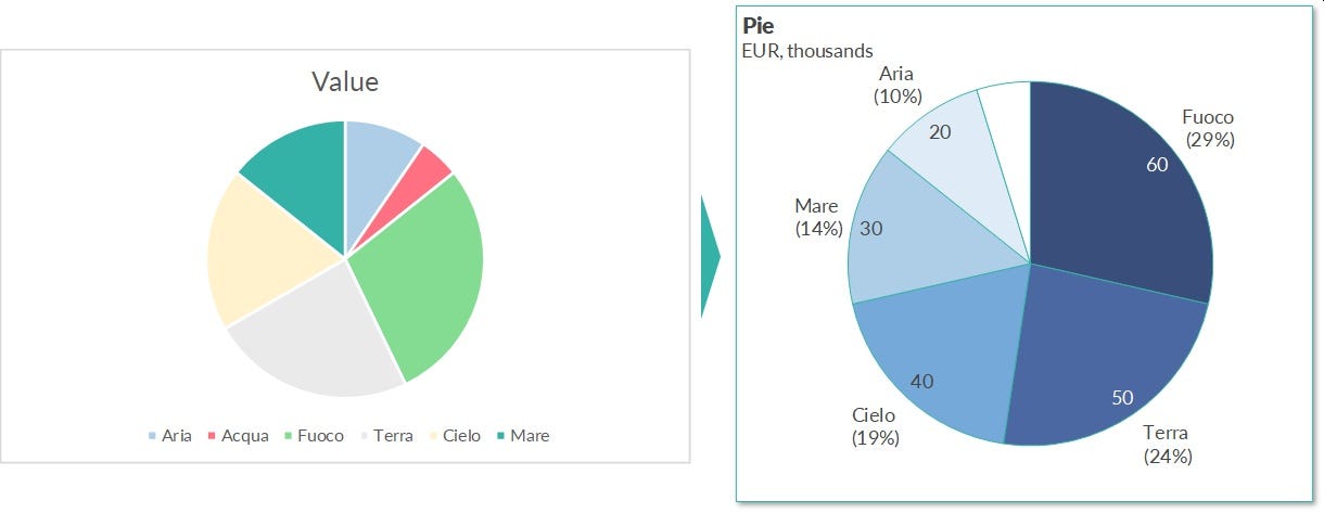
2.饼图 (2. Pie chart)

After pushing the Magic Button, to get the double labels, inside and outside, use the =evoLabelsApplyPie() function.

按下魔术按钮后，要获取内部和外部的双标签，请使用= evoLabelsApplyPie()函数。

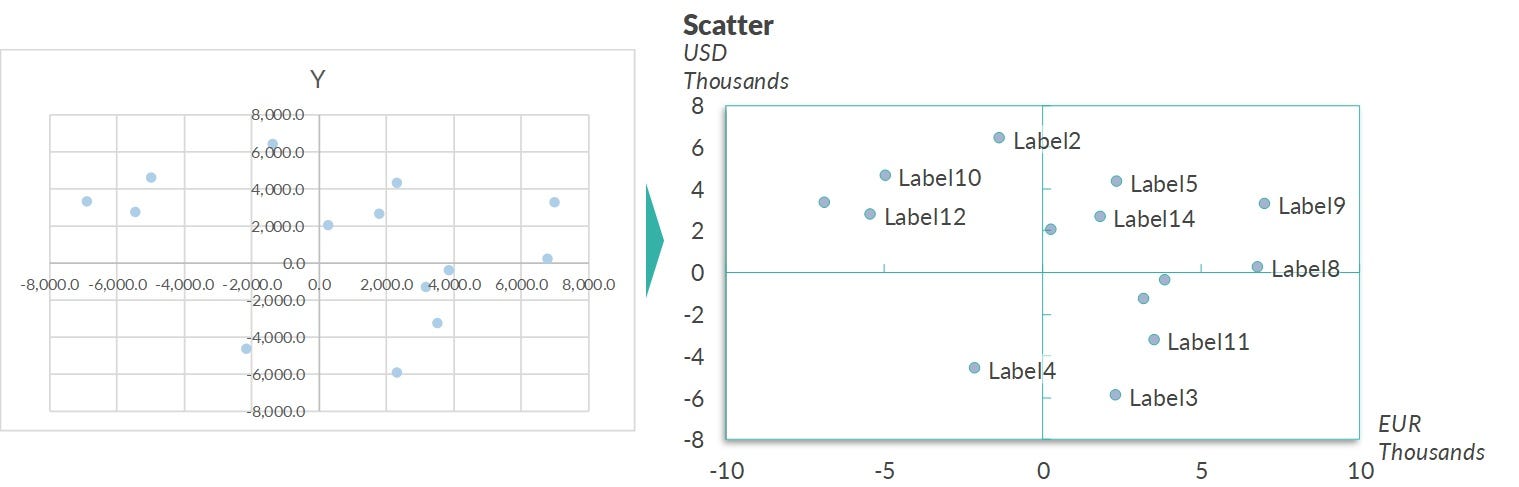
3.分散 (3. Scatter)

After pushing the Magic Button, format both the X and Y axes with the apply format function e.g.

按下魔术按钮后，使用套用格式化功能格式化X和Y轴，例如

=EvoChartApplyFormatCode(J16,EvoFormatCode(O15),”X”)

= EvoChartApplyFormatCode(J16，EvoFormatCode(O15)，“ X”)

to prevent all those unnecessary ,000,000,000 from crowding up the chart.

以防止所有不必要的000,000,000挤满图表。

Use =EvoLabelsHide() to remove overlapping labels.

使用= EvoLabelsHide()删除重叠的标签。

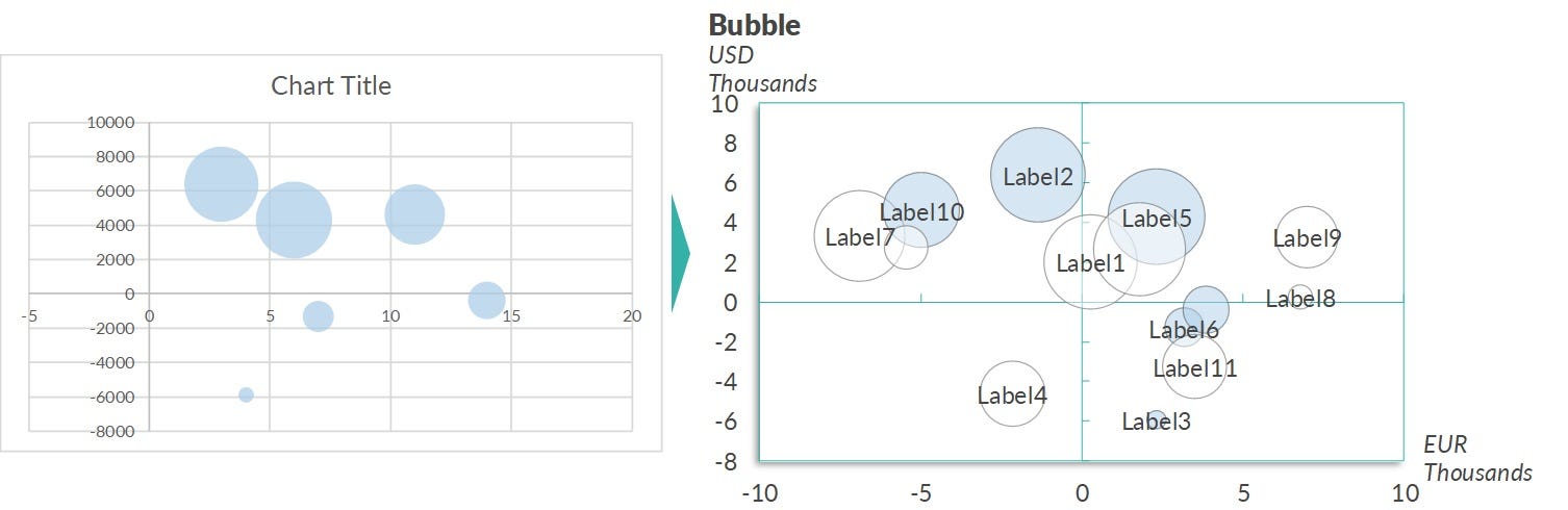
4.泡泡 (4. Bubble)

Same as the scatter chart, plus use positive/negative bubble sizes to have two different fills while using a single dataset.

与散点图相同，此外，在使用单个数据集时，请使用正/负气泡大小来填充两个不同的填充。

5.梯子 (5. Ladder)

Handy chart type to show price ranges; a bubble chart but with custom axis labels and vertical lines.

方便的图表类型以显示价格范围；气泡图，但带有自定义轴标签和垂直线。

6.专栏 (6. Column)

Truly handy chart for business!

真正方便的商务图表！

Pre-sort the data for greater readability using =evoSortValue() where relevant; hide labels of data sets smaller than 6% of the chart height by formatting a supporting dataset with =EvoChartApplyFormatCode().

在相关位置使用= evoSortValue()对数据进行预排序以提高可读性；通过使用= EvoChartApplyFormatCode()格式化支持的数据集来隐藏小于图表高度6％的数据集的标签。

7.箱线图 (7. Boxplot)

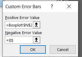
Regular column chart, where the base bar is hidden and the whiskers are error lines. Use to show distributions, e.g. of prices.

常规柱形图，其中基条被隐藏，而晶须是误差线 。用于显示价格的分布。

Note: custom error bars do not accept ‘empty’; if needed use ={0}

注意：自定义错误栏不接受“空”；如果需要，请使用= {0}

8.集群 (8. Clustered)

Not very readable. Use this chart type rarely, please :-)

不太可读。很少使用此图表类型，请:-)

9.酒吧 (9. Bar)

Use the Column chart as reference: the bar chart is a close relative!

使用柱形图作为参考：条形图是近亲！

源代码：Magic Button(如果不进行编程，则直接跳至下一部分！) (Source code: Magic Button (skip directly to the next section if not into programming!))

This is a Visual Basic C# / .NET project.

这是一个Visual Basic C＃/ .NET项目。

First, this first block of code behind the ‘Magic Button’ sets core properties, then calls the appropriate sub-function for the selected chart type; see below for further details.

首先，“魔术按钮”后面的第一段代码设置了核心属性，然后为选定的图表类型调用适当的子功能。有关更多详细信息，请参见下文。

public static void FormatMagicButton(Chart chart)
        {
            if (chart == null)
            {
                return;
            }// General
            chart.Parent.Placement = XlPlacement.xlMove;// ChartArea Font
            chart.ChartArea.Format.TextFrame2.TextRange.Font.Name = "Lato";
            chart.ChartArea.Format.TextFrame2.TextRange.Font.Size = 10;
            chart.ChartArea.Font.Color = FormatColors.EvoChartFont;// Shapes Font
            foreach (Shape shape in chart.Shapes)
            {
                shape.TextFrame2.TextRange.Font.Name = "Lato";
                shape.TextFrame2.TextRange.Font.Size = 10;
                shape.TextFrame2.TextRange.Font.Fill.ForeColor.RGB =
                    ColorTranslator.ToOle(FormatColors.EvoChartFont);
                shape.TextFrame2.TextRange.Font.Italic = MsoTriState.msoTrue;
            }// Title Font
            if (!chart.HasTitle)
            {
                chart.SetElement(Microsoft.Office.Core.MsoChartElementType.msoElementChartTitleAboveChart);
            }
            chart.ChartTitle.Position = XlChartElementPosition.xlChartElementPositionCustom;
            chart.ChartTitle.Left = chart.ChartTitle.Top = -3;
            chart.ChartTitle.Format.TextFrame2.TextRange.Font.Name = "Lato Black";
            chart.ChartTitle.Format.TextFrame2.TextRange.Font.Size = 12;
            chart.ChartTitle.Format.TextFrame2.TextRange.Font.Bold = MsoTriState.msoTrue;
            chart.ChartTitle.Font.Color = FormatColors.EvoChartFont;switch (chart.ChartType)
            {
                case XlChartType.xl3DBarClustered:
                case XlChartType.xl3DBarStacked:
                case XlChartType.xl3DBarStacked100:
                case XlChartType.xlBarClustered:
                case XlChartType.xlBarStacked:
                case XlChartType.xlBarStacked100:
                    FormatChartAreaBase(chart);
                    FormatBarChart(chart);
                    break;case XlChartType.xlBubble:
                case XlChartType.xlBubble3DEffect:
                    FormatPlotAreaBase(chart);
                    FormatBubbleChart(chart);
                    break;case XlChartType.xlColumnClustered:
                case XlChartType.xlColumnStacked:
                case XlChartType.xlColumnStacked100:
                case XlChartType.xl3DColumn:
                case XlChartType.xl3DColumnClustered:
                case XlChartType.xl3DColumnStacked:
                case XlChartType.xl3DColumnStacked100:
                    FormatChartAreaBase(chart);
                    FormatColumnChart(chart);
                    break;case XlChartType.xlLine:
                case XlChartType.xlLineStacked:
                case XlChartType.xlLineStacked100:
                case XlChartType.xlLineMarkers:
                case XlChartType.xlLineMarkersStacked:
                case XlChartType.xlLineMarkersStacked100:
                case XlChartType.xl3DLine:
                    FormatChartAreaBase(chart);
                    FormatLineChart(chart);
                    break;case XlChartType.xl3DPie:
                case XlChartType.xl3DPieExploded:
                case XlChartType.xlPie:
                case XlChartType.xlPieExploded:
                    FormatChartAreaBase(chart);
                    FormatPieChart(chart);
                    break;case XlChartType.xlXYScatter:
                case XlChartType.xlXYScatterLines:
                case XlChartType.xlXYScatterLinesNoMarkers:
                case XlChartType.xlXYScatterSmooth:
                case XlChartType.xlXYScatterSmoothNoMarkers:
                    FormatPlotAreaBase(chart);
                    FormatScatterChart(chart);
                    break;
            }

源代码：折线图格式 (Source code: Line chart formatting)

After the global function above, the specific code for the line chart (and any other chart type) is then relatively straightforward: scripting each chart property one line at a time, rather than applying them manually.

在上面的全局功能之后，折线图(和任何其他图表类型)的特定代码就相对简单了：一次为每个图表属性编写一行脚本，而不是手动应用它们。

private static void FormatLineChart(Chart chart)
	{// Axis X
		if (!chart.HasAxis[XlAxisType.xlCategory])
		{
			chart.SetElement(Microsoft.Office.Core.MsoChartElementType.msoElementPrimaryCategoryAxisShow);
		}
		var axisX = (Axis)chart.Axes(XlAxisType.xlCategory);
		axisX.TickLabels.Offset = 0;
		axisX.TickLabelPosition = XlTickLabelPosition.xlTickLabelPositionLow;
		axisX.TickLabels.Orientation = XlTickLabelOrientation.xlTickLabelOrientationHorizontal;
		axisX.MajorTickMark = XlTickMark.xlTickMarkInside;
		axisX.MinorTickMark = XlTickMark.xlTickMarkNone;
		axisX.Border.Color = FormatColors.EvoChartAxisBorder;
		axisX.Format.Line.Weight = .25f;
		axisX.Crosses = XlAxisCrosses.xlAxisCrossesMaximum;
		axisX.AxisBetweenCategories = false;
		axisX.MajorGridlines.Format.Line.Visible = MsoTriState.msoFalse;// Axis Y
		if (!chart.HasAxis[XlAxisType.xlValue])
		{
			chart.SetElement(Microsoft.Office.Core.MsoChartElementType.msoElementPrimaryValueAxisShow);
		}
		var axisY = (Axis)chart.Axes(XlAxisType.xlValue);
		axisY.TickLabels.Offset = 0;
		axisY.TickLabelPosition = XlTickLabelPosition.xlTickLabelPositionHigh;
		axisY.MajorTickMark = XlTickMark.xlTickMarkInside;
		axisY.MinorTickMark = XlTickMark.xlTickMarkNone;
		axisY.Border.Color = FormatColors.EvoChartAxisBorder;
		axisY.Format.Line.Weight = .25f;
		axisY.Crosses = XlAxisCrosses.xlAxisCrossesAutomatic;
		axisY.MajorGridlines.Format.Line.Visible = MsoTriState.msoFalse;// Series
		int seriesIndex = 0;
		var allSeries = (SeriesCollection)chart.SeriesCollection();
		var legendSeries = new List<String>();
		foreach (Series series in allSeries)
		{
			if (series.Formula.Contains($@"""{series.Name}"""))
			{
				series.Delete();
				continue;
			}
			var seriesDefinition = _seriesDefinitions[seriesIndex++ % _seriesDefinitions.Count];
			series.Format.Line.ForeColor.RGB = ColorTranslator.ToOle(seriesDefinition.Color);
			series.Format.Line.DashStyle = seriesDefinition.DashStyle;
			series.Format.Line.Weight = seriesDefinition.Weight;
			series.PlotOrder = allSeries.Count - seriesIndex + 1;
			if (legendSeries != null)
			{
				legendSeries.Add(series.Name);
			}
		}// Legend
		if (chart.HasLegend)
		{
			chart.Legend.Delete();
		}
		chart.SetElement(Microsoft.Office.Core.MsoChartElementType.msoElementLegendTop);
		chart.Legend.Left = chart.ChartArea.Width - chart.Legend.Width;
		chart.Legend.Top = 0;
		var legendHeight = chart.Legend.Height;var legends = (LegendEntries)chart.Legend.LegendEntries();
		try
		{
			int count = legends.Count;
			int i = 1;//remove legend entry from the chart
			while (count >= i)
			{
				legends.Item(i)?.Delete();
				i++;
			}
		}
		catch { }seriesIndex = 0;if (legendSeries.Any())
		{
			foreach (var name in legendSeries)
			{
				var series = allSeries.NewSeries();
				var seriesDefinition = _seriesDefinitions[seriesIndex++ % _seriesDefinitions.Count];
				series.Format.Line.ForeColor.RGB = ColorTranslator.ToOle(seriesDefinition.Color);
				series.Format.Line.DashStyle = seriesDefinition.DashStyle;
				series.Format.Line.Weight = seriesDefinition.Weight;
				series.Name = name;
				try
				{
					if (legends.Count > seriesIndex)
					{
						chart.Legend.LegendEntries(1)?.Delete();
					}
				}
				catch { }
			}
		}// PlotArea
		chart.PlotArea.Top = Math.Max(legendHeight, chart.ChartTitle.Height) + 10;
		chart.PlotArea.Height = chart.ChartArea.Height - chart.PlotArea.Top - 5;
		chart.PlotArea.Left = 30;
		chart.PlotArea.Width = chart.ChartArea.Width - chart.PlotArea.Left - 5;
}

奖金：准备测试的插件 (Bonus: ready-to-test add-in)

If, like me, you just want the ready solution without having to bother with code, here are the 3 simple steps to charting with zero effort:

如果像我一样，如果您只想使用现成的解决方案而不必去理会代码，那么这里是三个简单的步骤，可以轻松实现图表制作：

1- Download the Excel add-in installer
2- Activate your free account
3- Test the Magic Button

This comes with the Magic Button as well as 46 User Defined Functions, just start typing =evo inside any cell to get the full list.

它带有魔术按钮以及46个用户定义函数，只需在任何单元格内开始键入= evo即可获取完整列表。

Happy charting!

祝您图表愉快！

PS For more details about the rationale of each formatting choice, please review my related piece:

附注：有关每种格式选择的原理的更多详细信息，请查看我的相关文章：

Example results from using this approach:

使用此方法的示例结果：

翻译自: https://towardsdatascience.com/how-to-draw-9-professional-chart-types-with-zero-effort-c9eee6d2a9cc

前端绘制绘制图表

weixin_26750481

关注

0
点赞
踩
0

收藏

觉得还不错? 一键收藏
0
评论
前端绘制绘制图表_如何轻松地绘制9种专业图表类型

前端绘制绘制图表数据可视 (DATA VIZ)In this article, I share all tricks of the trade how I draw professional charts every day with minimal effort. 在本文中，我分享了所有交易技巧，如何每天以最小的努力绘制专业图表。 Detailed instructions and cor...
复制链接

扫一扫