


列主序好和行主序相乘
深度学习并不总是大数据问题的答案 (Deep learning is not always the answer to a big data problem)
Often times in the workplace, business stakeholders and managers associate machine learning and big data with deep learning. They will often think that the best solution to all data problems is deep learning, AI or neural networks or some combination of the prior (insert your favourite buzzword). As someone with a statistics background, I find this view quite frustrating as the type of machine learning algorithm chosen should be based upon five key considerations:
通常,在工作场所中,业务利益相关者和经理会将机器学习和大数据与深度学习相关联。 他们通常会认为,解决所有数据问题的最佳解决方案是深度学习,AI或神经网络或上述的某种组合(插入您喜欢的流行词)。 作为具有统计学背景的人,我发现这种观点令人沮丧,因为选择的机器学习算法的类型应基于五个关键考虑因素:
选择机器学习算法时的5个关键注意事项 (5 Key Considerations when selecting a machine learning algorithm)
- Type of data problem — i.e. supervised vs unsupervised 数据问题的类型-即有监督还是无监督
- The variable types within the dataset — i.e. categorical or numerical 数据集中的变量类型-即分类或数字
- The validation of underlying assumptions of the statistical model 验证统计模型的基本假设
- The resulting model accuracy 结果模型精度
The balance between precision vs. recall and sensitivity vs. specificity (for classification)
精度与召回率之间的平衡以及灵敏度与特异性之间的平衡( 用于分类 )
In the next few sections and over a couple of blog posts, I am going to go through the different types of models for supervised learning and apply the above considerations to each one.
在接下来的几节中,以及在几篇博客文章中,我将介绍用于监督学习的不同类型的模型,并将以上考虑因素应用于每个模型。
监督学习 (Supervised learning)
Most of the time, data problems require the application of supervised learning. This is when you know exactly what you want to predict — the target or dependent variable, and have a set of independent or predictor variables that you want to better understand in terms of their influence on the target variable. Then, the selection of a model is based on mapping the underlying pattern in the data to a function which is dependent upon the data’s distribution and variable types.
大多数情况下,数据问题需要应用监督学习。 在这种情况下,您可以确切地知道要预测什么- 目标变量或因变量 ,并具有一组希望根据其对目标变量的影响来更好地理解的自变量或预测变量。 然后,模型的选择基于将数据中的基础模式映射到依赖于数据分布和变量类型的函数。
The name “supervised learning” is used to describe these types of models because the model learns the underlying pattern on a training set. The number of iterations/rounds determines the number of times the model has a chance to learn from its past. In each subsequent round, the model tries to improve on model accuracy (accuracy metric selected by user) based on what it has learnt in previous runs. The model stops running either after its maximum number of runs has been achieved or when it can no longer improve the model accuracy (specified by early stopping in some models).
名称“ 监督学习 ”用于描述这些类型的模型,因为该模型可以学习训练集上的基础模式。 迭代次数/回合次数确定了模型有机会从过去学习的次数。 在随后的每个回合中,模型都会根据先前运行中所学到的知识,尝试提高模型的准确性(用户选择的准确性指标)。 模型在达到最大运行次数后或不再能够提高模型精度时停止运行(在某些模型中通过提前停止来指定)。
There are two types of supervised learning algorithms as shown in the figure below where the type of outcome variable determines whether you select regression or classification.
监督学习算法有两种类型,如下图所示,其中结果变量的类型确定您选择回归还是分类。
Let’s delve into regression first.
让我们首先研究回归。
回归 (Regression)
It is common for people to think everything is a linear regression problem, but this is not the case. Regression algorithms have a very strict set of assumptions that have to be met in order for the final results to be statistically reliable (*Note: I did not write statistically significant).
人们通常认为一切都是线性回归问题,但事实并非如此。 回归算法 为了使最终结果在统计上可靠 ,必须满足一系列非常严格的假设( *注:我没有写出统计学上的显着性 )。
为什么要回归? (Why Regression?)
Regression analysis is a predictive algorithm that is often used in time series analysis and forecasting. This is because it models the underlying relationship between predictor variables and the dependent variable and determines how the variation in the values of the predictor variables explains the variation in the outcome variable.
回归分析是一种预测算法,经常在时间序列分析和预测中使用。 这是因为它对预测变量和因变量之间的基本关系进行建模,并确定预测变量值的变化如何解释结果变量的变化。
There are several types of regression algorithms, but I will focus on the ones below.
回归算法有几种类型,但下面我将重点介绍。

Before I explore the above regression techniques further. Let’s gain an understanding of the assumptions associated with regression techniques.
在我进一步探讨上述回归技术之前。 让我们了解与回归技术相关的假设。
回归假设 (Regression Assumptions)
Residuals of the regression line are normally distributed — To ensure that the result from the regression model are valid, the residuals (difference between observed and predicted values) should follow a normal distribution (with mean zero and constant standard deviation). The residuals are also called error terms and their distribution can be observed on a normal probability plot (Q-Q). If the majority of the residuals are located on the diagonal normality line, then we can assume their normality.
回归线的残差是正态分布的—为确保回归模型的结果有效, 残差 (观测值与预测值之间的差)应遵循正态分布(均值为零且标准偏差恒定)。 残差也称为误差项,可以在正态概率图(QQ)上观察其分布。 如果大多数残差位于对角正态性线上,那么我们可以假定它们的正态性。

2. Variables in the dataset come from normally distributed populations — all variables in the data should also arise from normally distributed populations. Typically, in statistics if the sample size is large enough, then normality can be assumed according to the Central Limit Theorem. In some textbooks it is also low as n = 30.
2.数据集中的变量来自正态分布的总体 —数据中的所有变量也应来自正态分布的总体。 通常,在统计中,如果样本量足够大,则可以根据中心极限定理假定正态性。 在某些教科书中,n = 30也很低。
3. Residuals are independent — This assumption is checked to avoid auto-correlation amongst the residuals. When auto-correlation is present within the dataset, it can lead to underestimating the standard error which in turn can make predictors look statistically significant even when they aren’t.
3.残差是独立的-检查此假设以避免残差之间的自相关 。 当数据集中存在自相关时,它可能导致低估标准误差,从而使预测变量即使在没有统计学意义的情况下也具有统计学意义。
The Durbin-Watson Test can be utilised to check for auto-correlation. The Null Hypothesis is that the residuals are not linearly auto-correlated. Durbin-Watson’s d can take on any value between 2 and 4, but rule of thumb values of d that are between 1.5 and 2.5 are are used to indicate lack of auto-correlation in the residuals.
Durbin-Watson检验可用于检查自相关。 零假设是残差不是线性自相关的。 Durbin-Watson的d可以取2到4之间的任何值,但是经验法则是d的值介于1.5和2.5之间,以指示残差中不存在自相关。
Note: The Durbin-Watson test can only vouch for linear auto-correlation between direct neighbors (first-order effects).
注意:Durbin-Watson检验只能保证直接邻居之间的线性自相关(一阶效应)。

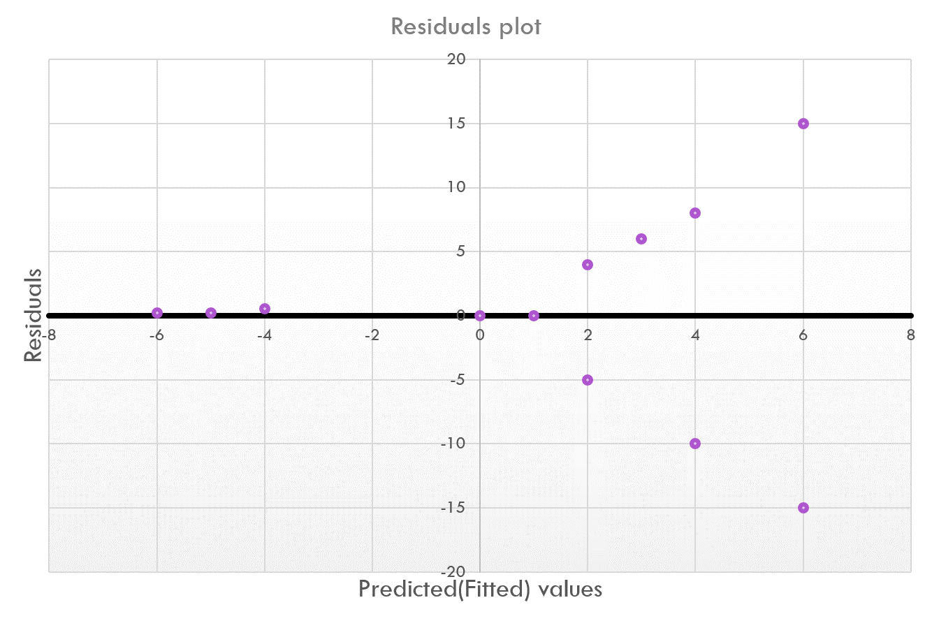
4. Data shows homoscedasticity — Homoscedasticity in the data occurs when the residuals are equally distributed along the line of best fit rather than show a pattern (residuals have constant variance). When heteroscedasticity is present, the shape of the residuals may show fanning (cone-like shape) or even a linear trend.
4.数据显示均方差—当残差沿着最佳拟合线均匀分布而不是显示出一种模式(残差具有恒定方差)时,数据就发生了均方差。 当存在异方差时,残差的形状可能呈扇形(圆锥形),甚至呈线性趋势。
Homoscedasticity can be assessed by plotting the residuals (y-axis) against the predicted values (x-axis) onto a scatterplot and looking for a random scatter of the points rather than any clusters or patterns. A statistical test for heteroscedascticity is the Goldfeld-Quandt Test. It involves dividing the dataset into two groups and checking to see if the variances of the residuals between the two groups are similar.
可以通过将残差(y轴)相对于预测值(x轴)绘制到散点图上并寻找点的随机散点(而不是任何聚类或图案)来评估均方差。 异方差性的统计检验是Goldfeld-Quandt检验 。 它涉及将数据集分为两组,并检查两组之间的残差方差是否相似。

5. Relationship is linear — When carrying out linear regression (simple or multiple), the relationship between the independent variable(s) and the dependent variable must be linear. Visually, this can be ascertained by creating a scatterplot between each independent variable and dependent variable pair and checking to see if there is a straight line that can be drawn through the points.
5.关系是线性的 -进行线性回归(简单或多元)时,自变量和因变量之间的关系必须是线性的。 在视觉上,可以通过在每个自变量和因变量对之间创建散点图并检查是否存在可以通过这些点绘制的直线来确定这一点。

5. There are no significant/influential outliers — Outliers are typically points within the dataset that are +/- 3 standard deviations from the mean or are beyond the whiskers of a boxplot. As outliers are extreme values they can have a significant effect on the slope of the best-fit line.
5. 没有显着/有影响的离群值 -离群值通常是数据集中的点,相对于平均值有+/- 3标准差或超出了箱线图的晶须。 由于离群值是极值,因此它们可能会对最佳拟合线的斜率产生重大影响。
- Outliers can be visually identified in boxplots (points that lie outside the whiskers) or from skewness in histograms. 异常值可以在箱图中(位于晶须之外的点)或直方图中的偏斜进行视觉识别。
To determine if the outliers are influential, there are two statistical metrics that can be used: 1) Cook’s Distance and 2) Mahanalobis Distance
要确定异常值是否具有影响力,可以使用两个统计量度: 1)库克距离和2)马哈那洛比斯距离
Cook’s Distance checks to see how the regression coefficients vary as each observation in the dataset is removed thereby checking their influence. Each value in the dataset is assigned a Cook’s Distance value. The larger the Cook’s distance, the more influential the observation. A typical heuristic used to determine if a value is an outlier is by checking to see if it’s Cook’s D value is greater than 4/n (where n is the size of the dataset).
Cook的距离检查可查看回归系数在删除数据集中每个观察值后如何变化,从而检查其影响。 数据集中的每个值都分配有一个库克距离值。 库克距离越大,观察的影响越大。 用于确定某个值是否为离群值的典型启发式方法是检查其Cook D值是否大于4 / n (其中n是数据集的大小)。
Mahanalobis Distance measures how far (how many standard deviations) is each observation from the majority of the data points (or mean) and is often used for multivariate datasets. This distance can be approximated using a chi-squared distribution with n degrees of freedom. Compute the p-value for each observation in the dataset. Check to see if the p-value is less than the level of significance (i.e. 0.01) to determine if they are extreme.
Mahanalobis距离用于测量每个观测值与大多数数据点(或均值)之间的距离 (多少个标准偏差),通常用于多变量数据集。 可以使用具有n个自由度的卡方分布来近似此距离。 计算数据集中每个观测值的p值 。 检查p值是否小于显着性水平(即0.01),以确定它们是否极端。
6. There is no multicollinearity* amongst the independent variables — Multicollinearity occurs when the independent variables are related to each other. If this is the case, typically you want to include only one of the variables within the pair into the regression model. This assumption can be checked using three methods.
6. 没有多重*之间的独立变量 -当独立变量的相互关系发生多重共线性 。 如果是这种情况,通常您只希望将变量对中的一个变量包含到回归模型中。 可以使用三种方法检查该假设。
*Does not apply to simple linear regression
*不适用于简单的线性回归
Variance Inflation Factor (VIF): Variables are multicollinear if their VIF value is greater than 10.
方差膨胀因子(VIF):如果变量的VIF值大于10,则它们是多重共线性的。

Correlation Coefficient (r): Create a correlation matrix between all pairs of variables. If the correlation coefficient is greater than or equal to -/+ 0.7, the the variables are highly correlated.
相关系数(r) :在所有变量对之间创建一个相关矩阵。 如果相关系数大于或等于-/ + 0.7,则变量高度相关。
Tolerance — This metric measures the how each independent variable influences all the other independent variables and is defined by the equation T = 1 — R-squared. R-squared (Coefficient of Determination) can be calculated for each independent variable by regressing it against the remaining independent variables. A tolerance factor of 0.1 is commonly used, where when T < 0.1, this indicates the presence of multicollinearity in the dataset.
公差 -此度量标准衡量每个自变量如何影响所有其他自变量,并由等式T = 1-R平方定义 。 可以通过将每个自变量相对于其余自变量进行回归来计算R平方(确定系数)。 通常使用0.1的公差系数,其中当T <0.1时 ,表明数据集中存在多重共线性。
回归假设回顾 (Recap of Regression Assumptions)
Let’s test some of the concepts we have learnt by running regression diagnostics on the Boston Housing data.
让我们测试通过对Boston Housing数据进行回归诊断所学到的一些概念。

Residuals vs Fitted — This plot is used to check for linearity. Given that the line is horizontal without any distinct patterns, we can assume a linear relationship.
残差vs拟合-此图用于检查线性。 假设线是水平的,没有任何明显的模式,我们可以假设是线性关系。
Normal Q-Q. This plot is used to check for normality of residuals. As most of the residuals are on the diagonal line, this assumption is satisfied.
普通QQ 。 该图用于检查残差的正态性。 由于大多数残差在对角线上,因此可以满足此假设。
Scale-Location (or Spread-Location) — this plot is used to examine whether the variance of the residuals is homogeneous (homoscedastic). We are looking for a horizontal line with equally distributed residuals below and above this line. In this case, the line has some curvature which means we have some heteroscedascticity.
比例位置 (或扩展位置)—此图用于检查残差的方差是否均匀(均方差)。 我们正在寻找一条水平线,在该线的上方和下方都有均布的残差。 在这种情况下,线具有一定的曲率,这意味着我们具有异质折断性。
Residuals vs Leverage. This plot is used to determine influential observations or those that have leverage. The points that are labelled in the plot appear to be influential. By removing these, we may also resolve the heteroscedasctic problem as the same observations are labelled in the previous plot.
残差vs杠杆 。 该图用于确定有影响力的观察或具有影响力的观察。 图中标记的点似乎具有影响力。 通过删除这些,我们也可以解决异方差问题,因为在上图中标有相同的观察结果。
Now let’s look at statistics that are commonly used to evaluate model performance.
现在让我们看一下通常用于评估模型性能的统计数据。
评估模型性能 (Evaluating model performance)
There are a couple of metrics that can be used to measure the accuracy of a regression model. I have described the ones I have commonly used when building models.
有几个指标可用于衡量回归模型的准确性。 我已经描述了构建模型时常用的模型。
R-squared: The coefficient of determination measures how much variation in the outcome variable can be explained by the variation in the independent variables. Higher R-squared values are seen as being reflective of higher model accuracy. However, R-squared is not to be trusted when there are multiple predictors in the model. This is because each predictor influences the R-squared value. In these instances, it is more reliable to use the adjusted R-squared. When deciding whether or not to trust the R-squared value, subject matter expertise in the area is required. For instance, R-squared can be quite high (close to 90%) in controlled environments such as chemical plants; however, when modelling human behaviour, a high R-squared value can be representative of overfitting. In these instances, it is better to use any of the below metrics to validate your model.
R平方 :确定系数衡量结果变量中的多少变量可以由自变量中的变量解释。 较高的R平方值被视为反映了较高的模型精度。 但是,当模型中有多个预测变量时,将不信任R平方 。 这是因为每个预测变量都会影响R平方值。 在这些情况下,使用调整后的R平方更可靠。 在决定是否信任R平方值时,需要该领域的专业知识。 例如,在受控环境(例如化工厂)中, R平方可能会很高(接近90%)。 但是,在对人类行为进行建模时,较高的R平方值可以表示过拟合 。 在这些情况下,最好使用以下任何指标来验证模型。
RMSE (Root-Mean Squared Error): It is calculated as the squared root of the variance between the predicted and observed values (residuals). the lower the value, the better the model fit. RMSE is a better metric in some cases because it penalizes large errors (residuals).
RMSE(均方根误差):计算为预测值和观察值( 残差 )之间方差的平方根。 值越低,模型拟合越好。 在某些情况下, RMSE是更好的指标,因为它会惩罚较大的错误(残差)。
MAE (Mean Absolute Error):This metric is simpler than the RMSE and just sums the absolute value of the residuals. It is less influenced by outliers. Each residual has a proportionate contribution to the total error in the equation. Once again, lower values are better.
MAE(平均绝对误差):此度量标准比RMSE简单,仅将残差的绝对值求和。 它受异常值的影响较小。 每个残差对方程式中的总误差有成比例的贡献。 再一次,较低的值会更好。
We can finally delve into understanding the various types of regression algorithms.
我们最终可以深入了解各种回归算法。
最小二乘回归 (Least-squares regression)
Linear regression, also called, least-squares regression, uses independent variables to approximate the best fit line for the outcome variable. It is a weighted equation that tries to minimize the sum of squared differences and is denoted by the following equation, where y is the predicted dependent variable, each β is a coefficient corresponding to each independent variable or x, β₀ is the y-intercept, and e is the error term.
线性回归(也称为最小二乘回归)使用独立变量来近似结果变量的最佳拟合线。 它是一个试图最小化平方差之和的加权方程,并由以下方程式表示,其中y是预测的因变量,每个β是与每个独立变量对应的系数,或者x,β是y截距, e是误差项。

In simple linear regression, there is only one coefficient and one independent variable. A coefficient term (β) is added for each independent variable (x) included in multiple linear regression.
在简单线性回归中 ,只有一个系数和一个自变量。 为多元线性回归中包含的每个自变量( x)添加一个系数项( β) 。
解释线性回归方程 (Interpreting a linear regression equation)
Let’s start with the y-intercept or constant, β₀. It is the value predicted for y if all the independent variables (X) were zero. It is also typically the average value of the predicted y.
让我们从y截距或常数β₀开始。 如果所有自变量( X)均为零,则是y的预测值。 通常,它也是预测y的平均值。
For coefficients of continuous predictor variables, they are interpreted as follows. Keeping all other variables constant, for every 1 unit of increase in X₁, y will increase (if β₁ is positive) or decrease (if β₁ is negative) by β₁ units on average.
对于连续预测变量的系数 ,它们的解释如下。 保持所有其他变量恒定时,在X₁每增加1个单位的,Y将增加(如果β₁ 为正)或减少(如果β₁ 是负的)由平均β₁ 单元 。
Categorical independent variables are coded as 0 or 1 (dummy variables) for linear regression. So when interpreting their coefficient, which is the difference in the predicted value of y, a one unit difference is a representation of switching from one category to the other while keeping all other variables constant.
分类自变量被编码为0或1(虚拟变量)以进行线性回归。 因此,在解释它们的系数(即y的预测值的差异)时,一个单位的差异表示从一种类别切换到另一种类别,同时保持所有其他变量不变。
多项式回归 (Polynomial regression)
When the relationship between the independent variable and dependent variable is non-linear in nature and includes curvature, polynomial regression can be considered an option.
当自变量和因变量之间的关系本质上是非线性的并且包括曲率时,可以将多项式回归视为一种选择。

In the graph on the left, we can see that polynomial regression (to the order of 2) fits slightly better than straight line.
在左侧的图中,我们可以看到多项式回归(约为2阶)比直线拟合得更好。
A polynomial regression equation for each independent variable is expressed below. For each order that the variable is raised to, an additional term is added for the variable into the equation.
每个自变量的多项式回归方程式如下所示。 对于将变量升至的每个阶数,都会将变量的附加项添加到方程式中。
It can be tempting to continue to raise the equation to higher degree polynomials to get the best fit; however, this can lead to over-fitting. Overfitting occurs when an attempt is made to try and explain as many points as possible, including the random errors, in the dataset (i.e. training set) making it difficult to generalise for other datasets (i.e. test sets).
可能会继续将方程式提高到更高的多项式以获得最佳拟合。 但是,这可能导致过度拟合 。 当试图尝试解释数据集(即训练集)中的尽可能多的点(包括随机误差)时,就会出现过度拟合 ,从而难以对其他数据集(即测试集)进行概括。

逐步回归 (Stepwise Regression)
Stepwise regression likes its name involves adding (forward selection starting with no independent variables in the model) or removing (backward selection starting with a full model or all independent variables in the model) independent variables in the linear model to find the best subset of predictors for the dependent variable based on the model evaluation metric.
逐步回归就像它的名字一样,涉及在线性模型中添加(从模型中没有自变量开始的正向选择)或从模型中没有模型(从完整模型或所有自变量开始的向后选择)中查找最佳预测变量子集基于模型评估指标的因变量。
Forward selection stops when there is no longer an improvement in the model evaluation metric (i.e. R-squared stops increasing), whereas backward selection halts after the least influential (i.e. those that contribute to R-squared) independent variables have been removed.
当模型评估指标不再得到改善时, 前向选择即停止(即R平方停止增加),而影响力最小的自变量(即有助于R平方的自变量)被删除后, 贝克选择停止。
R中的回归 (Regression in R)
线性回归 (Linear regression)
Sticking to the Boston housing dataset, I have run linear regression (“lm”) of all predictor variables against the median house price. Please note, that I did not “deal” with the multicollinearity, normality, and outlier issues prior to running the model.
坚持波士顿住房数据集,我对所有预测变量对中位数房价进行了线性回归(“ lm”)。 请注意,在运行模型之前,我没有“应对”多重共线性,正态性和异常问题。
> linearMod <- lm(medv ~ ., data=Boston)
> summary(linearMod)Call:
lm(formula = medv ~ ., data = Boston)Residuals:
    Min      1Q  Median      3Q     Max
-15.595  -2.730  -0.518   1.777  26.199Coefficients:
              Estimate Std. Error t value Pr(>|t|)
(Intercept)  3.646e+01  5.103e+00   7.144 3.28e-12 ***
crim        -1.080e-01  3.286e-02  -3.287 0.001087 **
zn           4.642e-02  1.373e-02   3.382 0.000778 ***
indus        2.056e-02  6.150e-02   0.334 0.738288
chas         2.687e+00  8.616e-01   3.118 0.001925 **
nox         -1.777e+01  3.820e+00  -4.651 4.25e-06 ***
rm           3.810e+00  4.179e-01   9.116  < 2e-16 ***
age          6.922e-04  1.321e-02   0.052 0.958229
dis         -1.476e+00  1.995e-01  -7.398 6.01e-13 ***
rad          3.060e-01  6.635e-02   4.613 5.07e-06 ***
tax         -1.233e-02  3.760e-03  -3.280 0.001112 **
ptratio     -9.527e-01  1.308e-01  -7.283 1.31e-12 ***
black        9.312e-03  2.686e-03   3.467 0.000573 ***
lstat       -5.248e-01  5.072e-02 -10.347  < 2e-16 ***
---
Signif. codes:  0 ‘***’ 0.001 ‘**’ 0.01 ‘*’ 0.05 ‘.’ 0.1 ‘ ’ 1Residual standard error: 4.745 on 492 degrees of freedom
Multiple R-squared:  0.7406, Adjusted R-squared:  0.7338
F-statistic: 108.1 on 13 and 492 DF,  p-value: < 2.2e-16
Above, we can see that the adjusted R-squared value is 73.38%, which means that this amount of variation in the median house price can be explained by the predictor variables in the model. This is a pretty good R-squared value and the p-value < 0.05 indicating statistical significance.
在上面,我们可以看到调整后的R平方值为73.38% ,这意味着房价中位数的这种变化量可以通过模型中的预测变量来解释。 这是一个相当不错的R平方值, p值<0.05表示具有统计学意义。
Next, I would determine which variables contribute to this R-squared statistic. I can see that all except indus and age are non-significant contributors (p-values > 0.05).
接下来,我将确定哪些变量有助于此R平方统计量。 我可以看到,除了梧桐和年龄之外,其他所有贡献都不重要(p值> 0.05)。
Let’s see what happens if I run stepwise regression.
让我们看看如果运行逐步回归会发生什么。
逐步回归 (Stepwise regression)
Backward
落后
Let’s try and interpret the call to the the model first.
让我们先尝试解释对模型的调用。
- My dependent variable (medv) has been regressed against all independent variables (.) 我的因变量(medv)已针对所有自变量(。)回归
- I have used backward regression 我已经使用了向后回归
- The model is going to be tuned to try models consisting of 1 to 13 variables. 该模型将被调整为尝试由1到13个变量组成的模型。
# Set seed for reproducibility
> set.seed(123)
> # Set up repeated k-fold cross-validation (10 fold)
> train.control <- trainControl(method = "cv", number = 10)
> # Train the model
> step.model <- train(medv ~ ., data=Boston,
+                     method = "leapBackward",
+                     tuneGrid = data.frame(nvmax = 1:13),
+                     trControl = train.control
+ )
> step.model$results
   nvmax     RMSE  Rsquared      MAE    RMSESD RsquaredSD     MAESD
1      1 6.190699 0.5542196 4.512277 0.6480792 0.03585104 0.5143497
2      2 5.537331 0.6393649 3.975099 0.6194193 0.08470812 0.4184383
3      3 5.216943 0.6757786 3.675974 0.7844579 0.09606216 0.3282287
4      4 5.144946 0.6843838 3.621869 0.6838151 0.08435306 0.3033078
5      5 4.998163 0.7010740 3.543459 0.7416779 0.08756225 0.2999431
6      6 5.048162 0.6953426 3.520865 0.7245789 0.08673190 0.2717374
7      7 5.049469 0.6952020 3.500608 0.6987592 0.08276566 0.2597508
8      8 5.008368 0.7004709 3.497253 0.6740135 0.08021108 0.2756674
9      9 5.012961 0.7018661 3.490065 0.6963818 0.08564270 0.2683468
10    10 4.947244 0.7098667 3.447318 0.6896883 0.08705085 0.222294311    11 4.809318 0.7249622 3.359429 0.6861143 0.08341394 0.2409937
12    12 4.825967 0.7231964 3.365846 0.6808653 0.08309689 0.2442360
13    13 4.829796 0.7227732 3.368084 0.6796633 0.08336179 0.2455718
> step.model$bestTune
   nvmax
11    11> summary(step.model$finalModel)
Subset selection object
13 Variables  (and intercept)
        Forced in Forced out
crim        FALSE      FALSE
zn          FALSE      FALSE
indus       FALSE      FALSE
chas        FALSE      FALSE
nox         FALSE      FALSE
rm          FALSE      FALSE
age         FALSE      FALSE
dis         FALSE      FALSE
rad         FALSE      FALSE
tax         FALSE      FALSE
ptratio     FALSE      FALSE
black       FALSE      FALSE
lstat       FALSE      FALSE
1 subsets of each size up to 11
Selection Algorithm: backward
          crim zn  indus chas nox rm  age dis rad tax ptratio black lstat
1  ( 1 )  " "  " " " "   " "  " " " " " " " " " " " " " "     " "   "*"
2  ( 1 )  " "  " " " "   " "  " " "*" " " " " " " " " " "     " "   "*"
3  ( 1 )  " "  " " " "   " "  " " "*" " " " " " " " " "*"     " "   "*"
4  ( 1 )  " "  " " " "   " "  " " "*" " " "*" " " " " "*"     " "   "*"
5  ( 1 )  " "  " " " "   " "  "*" "*" " " "*" " " " " "*"     " "   "*"
6  ( 1 )  " "  " " " "   " "  "*" "*" " " "*" " " " " "*"     "*"   "*"
7  ( 1 )  " "  " " " "   " "  "*" "*" " " "*" "*" " " "*"     "*"   "*"
8  ( 1 )  "*"  " " " "   " "  "*" "*" " " "*" "*" " " "*"     "*"   "*"
9  ( 1 )  "*"  " " " "   " "  "*" "*" " " "*" "*" "*" "*"     "*"   "*"
10  ( 1 ) "*"  "*" " "   " "  "*" "*" " " "*" "*" "*" "*"     "*"   "*"
11  ( 1 ) "*"  "*" " "   "*"  "*" "*" " " "*" "*" "*" "*"     "*"   "*"
In the example above, I have run backwards stepwise regression with 10-fold cross-validation and 13 maximum variables. I didn’t use all of them because we know two were not significant from running a full-linear model previously. We can see that the best model consists of 11 variables (lowest RMSE, lowest MAE, and highest R-squared).
在上面的示例中,我使用10倍交叉验证和13个最大变量进行了逐步回归。 我并没有全部使用它们,因为我们知道,从先前运行的全线性模型来看,其中两个并不重要。 我们可以看到,最佳模型包含11个变量(最低RMSE,最低MAE和最高R平方)。
The asterisk (*) indicates that a variable was included in the corresponding model. The best 11-variables model includes all variables except indus and age, just like the full linear model.
星号(*)表示变量已包含在相应的模型中。 像完整线性模型一样,最佳的11变量模型包括印度河和年龄以外的所有变量。
Forward stepwise regression gives us similar results to the full linear model and backward regression.
前向逐步回归给我们提供的结果与全线性模型和后向回归相似。
> set.seed(123)
> train.control <- trainControl(method = "cv", number = 10)
> step.model <- train(medv ~ ., data=Boston,
+                     method = "leapForward",
+                     tuneGrid = data.frame(nvmax = 1:13),
+                     trControl = train.control
+ )
> step.model$results
   nvmax     RMSE  Rsquared      MAE    RMSESD RsquaredSD     MAESD
1      1 6.190699 0.5542196 4.512277 0.6480792 0.03585104 0.5143497
2      2 5.537331 0.6393649 3.975099 0.6194193 0.08470812 0.4184383
3      3 5.216943 0.6757786 3.675974 0.7844579 0.09606216 0.3282287
4      4 5.243481 0.6736566 3.658219 0.7510340 0.08224804 0.3304744
5      5 5.098698 0.6904107 3.568604 0.7354806 0.08392928 0.2726078
6      6 5.045755 0.6953140 3.512300 0.7223225 0.08606320 0.2787373
7      7 4.969144 0.7036333 3.448631 0.7542104 0.08842114 0.2944921
8      8 4.985899 0.7027153 3.456932 0.7099500 0.08432911 0.2895184
9      9 4.985690 0.7030156 3.466382 0.6879376 0.08295944 0.2782166
10    10 4.912877 0.7137519 3.421565 0.6865803 0.07813425 0.2716994
11    11 4.809318 0.7249622 3.359429 0.6861143 0.08341394 0.2409937
12    12 4.825967 0.7231964 3.365846 0.6808653 0.08309689 0.2442360
13    13 4.829796 0.7227732 3.368084 0.6796633 0.08336179 0.2455718
> step.model$bestTune
   nvmax
11    11
正则化 (Regularization)
Regularization is a technique that is often used to solve the over-fitting and multicollinearity issues that may occur with regression. It does this via the addition of a penalty term to the objective function which aims to reduce standard error.
正则化是一种通常用于解决回归过程中可能出现的过拟合和多重共线性问题的技术。 它通过在目标函数中增加一个惩罚项来减少标准误差,从而实现这一目的。
岭回归 (Ridge Regression)
In ridge regression, a penalty term (shrinkage parameter), λ, is added to reduce the large variation in the β coefficient terms. L2 regularization is used in ride regression, where the objective is to minimize the sum of squares of coefficients by trying to bring the coefficients closer to zero.
在岭回归中,增加了惩罚项(收缩参数)λ,以减少β系数项的较大变化。 L2正则化用于平顺性回归,其目的是通过尝试使系数接近零来最小化系数平方和 。
Ridge regression is good for small datasets with a large number of variables with small to medium effect.
Ridge回归适用于具有大量变量的小型数据集,影响程度从小到中。
套索回归 (Lasso Regression)
Lasso (Least Absolute Shrinkage and Selection Operator) regression uses L1 regularization where λ is added to the sum of absolute squares of the coefficients.
Lasso(最小绝对收缩和选择算子)回归使用L1正则化 ,其中λ被添加到系数的绝对平方和。
Lasso regression is good for datasets with fewer variables with medium to large effect on the dependent variable.
套索回归适用于变量较少,对因变量影响中等到较大的数据集。
ElasticNet回归 (ElasticNet Regression)
ElasticNet combines both Lasso and Ridge Regression techniques where both L1 and L2 regularization are applied.
ElasticNet结合了套索和岭回归技术,其中同时应用了L1和L2正则化。
选择正则化参数 (Selecting the Regularization Parameter)
When deciding on which regularization parameter to use, we can base this on two methods — 1) where we choose λ where the information criterion is minimised (such as AIC or BIC) focusing on model fit or 2) where we run the model with cross-validation and select the value of λ that minimize the cross-validated residuals focusing on prediction accuracy.
在决定使用哪个正则化参数时,我们可以基于两种方法-1)选择信息准则最小化的λ(例如AIC或BIC),着重于模型拟合; 2)使用交叉模型运行模型。 -验证并选择λ的值,该值可最小化针对预测精度的交叉验证残差。
回归的利与弊 (Pros and Cons of Regression)
Pros
优点
- Easy to understand and present to stakeholders 易于理解并呈现给利益相关者
- Can be used for explainability — i.e relative influence of each predictor on outcome variable 可用于解释性,即每个预测变量对结果变量的相对影响
Cons
缺点
- Important to standardize (scale and center) all independent variables to avoid multicollinearity 标准化(缩放和居中)所有自变量以避免多重共线性很重要
- Requires checking of strict model assumptions 需要检查严格的模型假设
That was all I had on regression. My next blog post will be on classification algorithms.
那就是我回归的全部。 我的下一篇博客文章将介绍分类算法。
列主序好和行主序相乘


 762
762

 被折叠的 条评论
为什么被折叠?
被折叠的 条评论
为什么被折叠?
 到【灌水乐园】发言


