分类数据集的分析与探索_探索性数据流失数据集实用指南

分类数据集的分析与探索

Exploratory data analysis (EDA) is an essential part of the data science or the machine learning pipeline. In order to create a robust and valuable product using the data, you need to explore the data, understand the relations among variables, and the underlying structure of the data.

探索性数据分析(EDA)是数据科学或机器学习管道的重要组成部分。 为了使用数据创建强大而有价值的产品，您需要浏览数据，了解变量之间的关系以及数据的基础结构。

In this post, we will explore a customer churn dataset using Pandas, Matplotlib, and Seaborn libraries. The dataset is available here on Kaggle.

在本文中，我们将使用Pandas，Matplotlib和Seaborn库探索客户流失数据集。 该数据集可在这里上Kaggle。

The first step is to read the dataset into a pandas dataframe.

第一步是将数据集读入熊猫数据框。

import pandas as pd
import numpy as npdf = pd.read_csv("/content/Churn_Modelling.csv")df.shape
(10000, 14)df.head()

The dataset contains 10000 customers (i.e. rows) and 14 features about the customers and their products at a bank. The goal here is to predict whether a customer will churn (i.e. exited = 1) using the provided features. Thus, in terms of machine learning, we aim to build a supervised learning algorithm to perform a classification task.

该数据集包含10000个客户(即行)和银行中有关客户及其产品的14个特征。 这里的目标是使用提供的功能预测客户是否会流失(即退出= 1)。 因此，就机器学习而言，我们旨在构建一种监督学习算法来执行分类任务。

We should never just dump the raw data into a machine learning model. Garbage in, garbage out! That is the reason why a thorough EDA process is highly important.

我们绝不应该将原始数据转储到机器学习模型中。 垃圾进垃圾出！ 这就是彻底的EDA流程非常重要的原因。

清理数据 (Cleaning the data)

Let’s first check if there are any missing values.

我们首先检查是否存在任何缺失值。

df.isna().sum()

This dataset does not have any missing value which is not typical with real-life datasets. Handling missing values is an important part of the EDA process. If there are very few missing values compared to the size of the dataset, we may choose to drop rows that have missing values. Otherwise, it is better to replace them with appropriate values. Pandas fillna function can be used to handle this task.

该数据集没有任何缺失值，这在现实生活中是不常见的。 处理缺失值是EDA流程的重要组成部分。 如果与数据集的大小相比缺失值很少，我们可以选择删除具有缺失值的行。 否则，最好将它们替换为适当的值。 熊猫fillna函数可用于处理此任务。

Important note: If you choose to impute missing values based on the non-missing values in a column (e.g. fill missing values with the mean value of a column), you should do it after splitting your dataset into train and test subsets. Otherwise, you leak data to the machine learning model from the test set which is supposed to be new, previously unseen data.

重要说明：如果您选择根据一列中的非缺失值来估算缺失值(例如，用一列的平均值填充缺失值)，则应在将数据集拆分为训练和测试子集之后执行此操作。 否则，您会将数据从测试集中泄漏到机器学习模型中，该数据应该是新的，以前看不见的数据。

Tasks like churn prediction and email spam detection are likely to have an imbalance class distribution. The number of customers who churned (i.e. left) is usually much less than the number of customers who did not churn. We can check the distribution of values with the value_counts function.

流失预测和电子邮件垃圾邮件检测等任务很可能具有不平衡的类别分布。 流失(即离开)的客户数量通常比不流失的客户数量少得多。 我们可以使用value_counts函数检查值的分布。

df.Exited.value_counts()
0    7963 
1    2037 
Name: Exited, dtype: int64

There is an imbalance in the target variable (“Exited”). It is important to eliminate the imbalance. Otherwise, the machine learning model is likely to be biased towards the dominant class. There are different techniques to handle class imbalance such as undersampling and oversampling.

目标变量(“已退出”)不平衡。 消除不平衡很重要。 否则，机器学习模型可能会偏向主导阶层。 有多种技术可用于处理类不平衡问题，例如欠采样和过采样。

We should also make sure the data stored with appropriate data types. For instance, the numerical values should not be stored as “object”. Dtypes function returns the data type of each column.

我们还应确保以适当的数据类型存储数据。 例如，数值不应存储为“对象”。 Dtypes函数返回每一列的数据类型。

df.dtypes

The data types are appropriate. The next step is to get rid of redundant features. “RowNumber” column is just an index. “CustomerId” and “Surname” columns are obviously useless for a machine learning model. Thus, we should drop them.

数据类型是适当的。 下一步是摆脱冗余功能。 “ RowNumber”列只是一个索引。 “ CustomerId”和“ Surname”列对于机器学习模型显然毫无用处。 因此，我们应该丢弃它们。

df.drop(['RowNumber','CustomerId','Surname'], axis=1, inplace=True)

We just pass the list of labels to be dropped. The axis parameter tells the drop function if we are dropping rows (0) or columns (1). The inplace parameter is set as true to save the changes.

我们只是传递要删除的标签列表。 axis参数告诉drop函数是否要删除行(0)或列(1)。 inplace参数设置为true以保存更改。

更令人兴奋的部分！ (The more exciting part!)

It is time to dive deep into the dataset now.

现在是时候深入研究数据集了。

Let’s check how “Gender” and “Geography” are related to customer churn. One way is to use the groupby function of pandas.

让我们检查一下“性别”和“地理位置”与客户流失之间的关系。 一种方法是使用熊猫的groupby功能。

df[['Geography','Gender','Exited']].groupby(['Geography','Gender']).agg(['mean','count'])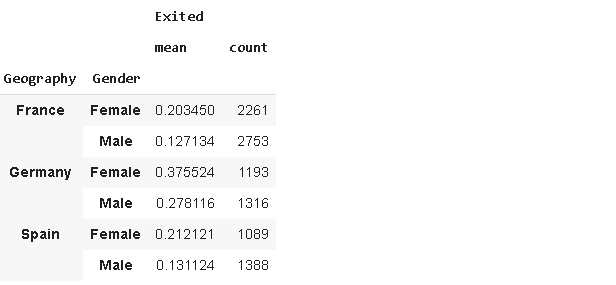

Finding: In general, females are more likely to “exit” than males. The exit (churn) rate in Germany is higher than in France and Spain.

结论 ：一般而言，女性比男性更有可能“退出”。 德国的退出率(流失率)高于法国和西班牙。

Another common practice in the EDA process is to check the distribution of variables. Distribution plots, histograms, and boxplots give us an idea about the distribution of variables (i.e. features).

EDA过程中的另一个常见做法是检查变量的分布。 分布图，直方图和箱形图使我们对变量(即特征)的分布有了一个想法。

fig , axs = plt.subplots(ncols=2, figsize=(12,6))fig.suptitle("Distribution of Balance and Estimated Salary", fontsize=15)sns.distplot(df.Balance, hist=False, ax=axs[0])sns.distplot(df.EstimatedSalary, hist=False, ax=axs[1])

Most of the customers have zero balance. For the remaining customers, the “Balance” has a normal distribution. The “EstimatedSalary” seems to have a uniform distribution.

大多数客户的余额为零。 对于其余客户，“余额”具有正态分布。 “估计工资”似乎有一个均匀的分布。

Since there are lots of customers with zero balance, We may create a new binary feature indicating whether a customer has zero balance. The where function of pandas will do the job.

由于有很多客户的余额为零，因此我们可能会创建一个新的二进制功能，指示客户是否具有零余额。 熊猫的where功能将完成这项工作。

df['Balance_binary'] = df['Balance'].where(df['Balance'] == 0, 1)df['Balance_binary'].value_counts()
1.0    6383 
0.0    3617 
Name: Balance_binary, dtype: int64

Approximately one-third of customers have zero balance. Let’s see the effect of having zero balance on churning.

大约三分之一的客户的余额为零。 让我们看看零搅拌对搅拌的影响。

df[['Balance_binary','Exited']].groupby('Balance_binary').mean()

Finding: Customers with zero balance are less likely to churn.

发现 ：余额为零的客户流失的可能性较小。

Another important statistic to check is the correlation among variables.

要检查的另一个重要统计数据是变量之间的相关性。

Correlation is a normalization of covariance by the standard deviation of each variable. Covariance is a quantitative measure that represents how much the variations of two variables match each other. To be more specific, covariance compares two variables in terms of the deviations from their mean (or expected) value.

相关性是每个变量的标准偏差对协方差的归一化。 协方差是一种定量度量，表示两个变量的变化相互匹配的程度。 更具体地说，协方差比较两个变量的平均值(或期望值)偏差。

By checking the correlation, we are trying to find how similarly two random variables deviate from their mean.

通过检查相关性，我们试图找到两个随机变量偏离其均值的相似程度。

The corr function of pandas returns a correlation matrix indicating the correlations between numerical variables. We can then plot this matrix as a heatmap.

熊猫的corr函数返回一个相关矩阵，指示数值变量之间的相关性。 然后，我们可以将该矩阵绘制为热图。

It is better if we convert the values in the “Gender” column to numeric ones which can be done with the replace function of pandas.

最好将“性别”列中的值转换为数字值，这可以通过熊猫的替换功能来完成。

df['Gender'].replace({'Male':0, 'Female':1}, inplace=True)corr = df.corr()plt.figure(figsize=(12,8))sns.heatmap(corr, cmap='Blues_r', annot=True)

The correlation matrix

相关矩阵

Finding: The “Age”, “Balance”, and “Gender” columns are positively correlated with customer churn (“Exited”). There is a negative correlation between being an active member (“IsActiveMember”) and customer churn.

结果 ：“年龄”，“平衡”和“性别”列与客户流失(“退出”)呈正相关。 成为活跃成员(“ IsActiveMember”)与客户流失之间存在负相关关系。

If you compare “Balance” and “Balance_binary”, you will notice a very strong positive correlation since we created one based on the other.

如果将“ Balance”和“ Balance_binary”进行比较，您会注意到一个非常强的正相关性，因为我们是基于另一个创建的。

Since “Age” turns out to have the highest correlation values, let’s dig in a little deeper.

由于事实证明“年龄”具有最高的相关值，因此让我们深入一点。

df[['Exited','Age']].groupby('Exited').mean()

The average age of churned customers is higher. We should also check the distribution of the “Age” column.

流失客户的平均年龄较高。 我们还应该检查“年龄”列的分布。

plt.figure(figsize=(6,6))plt.title("Boxplot of the Age Column", fontsize=15)sns.boxplot(y=df['Age'])

The dots above the upper line indicate outliers. Thus, there are many outliers on the upper side. Another way to check outliers is comparing the mean and median.

上线上方的点表示异常值。 因此，在上侧有许多离群值。 检查离群值的另一种方法是比较均值和中位数。

print(df['Age'].mean())
38.9218print(df['Age'].median())
37.0

The mean is higher than the median which is compatible with the boxplot. There are many different ways to handle outliers. It can be the topic of an entire post.

平均值高于与箱线图兼容的中位数。 有许多不同的方法可以处理异常值。 它可以是整个帖子的主题。

Let’s do a simple one here. We will remove the data points that are in the top 5 percent.

让我们在这里做一个简单的。 我们将删除前5％的数据点。

Q1 = np.quantile(df['Age'],0.95)df = df[df['Age'] < Q1]df.shape
(9474, 14)

The first line finds the value that distinguishes the top 5 percent. In the second line, we used this value to filter the dataframe. The original dataframe has 10000 rows so we deleted 526 rows.

第一行找到区分前5％的值。 在第二行中，我们使用此值来过滤数据帧。 原始数据帧有10000行，因此我们删除了526行。

Please note that this is not acceptable in many cases. We cannot just get rid of rows because data is a valuable asset and the more data we have the better models we can build. We are just trying to see if outliers have an effect on the correlation between age and customer churn.

请注意，在许多情况下这是不可接受的。 我们不能仅仅摆脱行，因为数据是宝贵的资产，而我们拥有的数据越多，我们可以建立的模型就越好。 我们只是想看看离群值是否会对年龄和客户流失之间的相关性产生影响。

Let’s compare the new mean and median.

让我们比较一下新的均值和中位数。

print(df['Age'].mean())
37.383681655055945print(df['Age'].median())
37.0

They are pretty close. It is time to check the difference between the average age of churned customers and those who did not churn.

他们非常接近。 现在该检查一下流失客户的平均年龄与未流失客户的平均年龄之间的差异了。

df[['Exited','Age']].groupby('Exited').mean()

Our finding still holds true. The average age of churned customers is higher.

我们的发现仍然成立。 流失客户的平均年龄较高。

There is no limit on exploratory data analysis. Depending on our task or goal, we can approach the data from a different perspective and dig deep to explore. However, the tools used in the process are usually similar. It is very important to practice a lot in order to get well in this process.

探索性数据分析没有限制。 根据我们的任务或目标，我们可以从不同的角度处理数据并进行深入研究。 但是，该过程中使用的工具通常是相似的。 为了使这个过程好起来，练习很多非常重要。

Thank you for reading. Please let me know if you have any feedback.

感谢您的阅读。 如果您有任何反馈意见，请告诉我。

翻译自: https://towardsdatascience.com/a-practical-guide-for-exploratory-data-analysis-churn-dataset-508b6da2d594

分类数据集的分析与探索