


Use of Bag of words technique & Random Forest algorithm to identify spam comments
使用词袋技术和随机森林算法识别垃圾邮件评论

As, you are on this page, I am assuming that you have completed your Machine Learning course & further looking to implement your skills.
就像您在此页面上一样,我假设您已经完成了机器学习课程,并且进一步寻求实现自己的技能。
Well then, “YouTube spam comment detector” is a great way to start & get your hands dirty.
那么,“ YouTube垃圾邮件评论检测器”是一种很好的开始方式,可以使您的双手变得肮脏。
前提条件 (PRE-REQUISITES)
> Familiarity with Python> Working knowledge of Random Forest algorithm and Bag of words model will be a plus. In any case, I will be explaining these terms as we move ahead
>熟悉Python>具有Random Forest算法和Bag of Words模型的工作知识将是一个加分。 无论如何,我将在前进的过程中解释这些术语
数据集 (THE DATA SET)
The dataset is pretty straightforward, it contains 2,000 comments from popular Youtube videos, The dataset is formatted in a way where each row has a comment followed by a value marked as 1 or 0 for spam or not spam,
该数据集非常简单,包含来自YouTube热门视频的2,000条评论,该数据集的格式设置为每一行都有评论,后跟一个标记为1或0的垃圾邮件或非垃圾邮件的值,
The dataset can be downloaded from this website
数据集可以从该网站下载
http://archive.ics.uci.edu/ml/datasets/YouTube+Spam+Collection
http://archive.ics.uci.edu/ml/datasets/YouTube+Spam+Collection
While on the website, click on the Data Folder directory, Scrolling below will give a brief description of the dataset.
在网站上时,单击“数据文件夹”目录,下面滚动将简要描述数据集。

Further ahead, click on the 2nd directory i.e, Youtube-Spam-Collection-v1 Extract all the files in a folder.
再往前,单击第二个目录,即Youtube-Spam-Collection-v1提取文件夹中的所有文件。
I
一世
The coding part will be performed in Spyder, although you are free to choose an IDE of your choice as long as it supports Python.
编码部分将在Spyder中执行,尽管您可以自由选择所需的IDE,只要它支持Python。
词袋 (Bag of words)
The bag-of-words model does exactly we want, that is to convert the phrases or sentences and counts the number of times a similar word appears. In the world of computer science, a bag refers to a data structure that keeps track of objects like an array or list does, but in such cases the order does not matter and if an object appears more than once, we just keep track of the count rather we keep repeating them.
词袋模型正是我们想要的,即转换短语或句子并计算相似词出现的次数。 在计算机科学世界中,包是指像数组或列表一样跟踪对象的数据结构,但是在这种情况下顺序并不重要,如果对象出现多次,我们只需跟踪而是我们会不断重复它们。
Consider the following sentences and try to find what makes the first pair of phrases similar to the second pair:
考虑以下句子,并尝试找出是什么使第一对短语与第二对相似:
As you can see, the first phrase from the diagram, has a bag of words that contains words such as “channel”, with one occurrence, “plz”, with one occurrence, “subscribe”, two occurrences, and so on. Then, we would collect all these counts in a vector, where one vector per phrase or sentence or document, depending on what you are working with. Again, the order in which the words appeared originally doesn’t matter.
如您所见,该图中的第一个短语包含一袋单词,其中包含诸如“ channel”,一个出现,“ plz”,一个出现,“ subscribe”,两个出现等的单词。 然后,我们将所有这些计数收集到一个向量中,其中每个短语,句子或文档一个向量,这取决于您使用的对象。 同样,单词最初出现的顺序无关紧要。
Further ahead, We make a larger vector with all the unique words across both phrases, we get a proper matrix representation. With each row representing a different phrase, notice the use of 0 to indicate that a phrase doesn’t have a word:
再往前,我们用两个短语中的所有唯一单词制作了一个更大的向量,我们得到了正确的矩阵表示。 每行代表一个不同的短语,请注意使用0表示短语没有单词:

If you want to have a bag of words with lots of phrases, documents, or we would need to collect all the unique words that occur across all the examples and create a huge matrix, N x M, where N is the number of examples and M is the number of occurrences
如果您想要一袋包含大量短语,文档的单词,或者我们需要收集所有示例中出现的所有唯一单词,并创建一个巨大的矩阵N x M,其中N是示例数, M是出现的次数
Additionally, there are some points which we need to take care about before preparing a bag of words model* Lowercase every word* Drop punctuation* Drop very common words (stop words)* Remove plurals (for example, bunnies => bunny)* Perform Lemmatization (for example, reader => read, reading = read)* Keep only frequent words (for example, must appear in >10 examples)* Record binary counts (1 = present, 0 = absent) rather than true counts
此外,在准备一袋单词模型之前,我们需要注意一些要点*小写每个单词*删除标点符号*删除非常常见的单词(停用词)*删除复数形式(例如,兔子=>兔子)*执行合法化(例如,阅读器=>读取,阅读=读取)*仅保留频繁的单词(例如,必须出现在> 10个示例中)*记录二进制计数(1 =存在,0 =不存在),而不是真实计数
Furthermore, if we still wanted to reduce very common words and highlight the rare ones, what we would need to do is record the relative importance of each word rather than its raw count. This is known as term frequency inverse document frequency (TF-IDF), which measures how common a word or term is in the document.
此外,如果我们仍然希望减少非常常见的单词并突出显示稀有单词,那么我们需要做的是记录每个单词的相对重要性,而不是其原始计数。 这称为术语频率逆文档频率 ( TF-IDF ),它测量单词或术语在文档中的普遍程度。
随机森林算法 (Random Forest Algorithm)
Random forests are extensions of decision trees and are a kind of ensemble method. Ensemble methods can achieve high accuracy by building several classifiers and running a each one independently. When a classifier makes a decision, you can make use of the most common and the average decision. If we use the most common method, it is called voting.
随机森林是决策树的扩展,是一种集成方法。 集成方法可以通过构建多个分类器并独立运行每个分类器来实现高精度。 当分类器做出决定时,您可以利用最常见和最平均的决定。 如果我们使用最常见的方法,则称为投票。
Here’s a diagram depicting the ensemble method:
这是描述合奏方法的图:

A random forest is a collection or ensemble of decision trees. Each tree is trained on a random subset of the attributes, as shown in the following diagram:
随机森林是决策树的集合或集合。 每棵树都在属性的随机子集上进行训练,如下图所示:

Consider using a random forest when there is a sufficient number of attributes to make trees and the accuracy is paramount. When there are fewer trees, the interpretability is difficult compared to a single decision tree.
当有足够多的属性可以制作树木并且精度至关重要时,请考虑使用随机森林。 当树数较少时,与单个决策树相比,其可解释性就很困难。
准备我们的代码 (Preparing our code)
Importing the dataset
导入数据集
First, we will import a single dataset. This dataset is actually split into four different files. Our set of comments comes from the PSY-Gangnam Style video:
首先,我们将导入一个数据集。 该数据集实际上分为四个不同的文件。 我们的评论来自PSY-Gangnam Style视频:
import matplotlib.pyplot as plt
import pandas as pd
df = pd.read_csv(‘D:\\Machine Learning_Algoritms\\Youtube-Spam-Check\\Youtube01-Psy.csv’, encoding =’latin1')
Now, if you are using Spyder, in the ‘Variable Explorer’ tab, you can check, if a variable ‘df ’ is created and assigned with the dataset, similiar to the one in the diagram below:
现在,如果您使用的是Spyder,则在“变量资源管理器”选项卡中,可以检查是否已创建变量“ df”并将其分配给数据集,与下图中的变量类似:

Checking for null values
检查空值
##checking for all the null valuesdf.isnull().sum()
Luckily, there are no missing values, so we can proceed ahead.
幸运的是,没有遗漏任何值,因此我们可以继续进行。
Look for the category distribution in categorical columns
在类别列中查找类别分布
Let’s look at the count of how many rows in the dataset are spam and how many are not spam
让我们看一下数据集中有多少行是垃圾邮件,有几行不是垃圾邮件的计数
##category distribution
df[‘CLASS’].value_counts()
The result we acquired is 175 and 175 respectively, which sums up to 350 rows overall in this file.
我们获得的结果分别为175和175,该文件中总共总计350行。
Bag of Words Technique
言语手法
In scikit-learn, the bag of words technique is actually called ‘CountVectorizer’, which means counting how many times each word appears and puts them into a vector. To create a vector, we need to make an object for ‘CountVectorizer’, and then perform the fit and transform simultaneously:
在scikit-learn中,单词袋技术实际上称为“ CountVectorizer”,这意味着计算每个单词出现的次数并将其放入向量中。 要创建向量,我们需要为“ CountVectorizer”创建一个对象,然后同时执行拟合和转换:
from sklearn.feature_extraction.text import CountVectorizer
vectorizer = CountVectorizer()
dv = vectorizer.fit_transform(df[‘CONTENT’])
This is performed in two different steps. First comes the fit step, where it discovers which words are present in the dataset, and second is the transform step, which gives you the bag of words matrix for those phrases
这是通过两个不同的步骤执行的。 首先是拟合步骤,它发现数据集中存在哪些单词,其次是转换步骤,为您提供这些短语的词袋矩阵
dv
There are 350 rows, which means we have 350 different comments and 1,482 words.
有350行,这意味着我们有350个不同的注释和1,482个单词。
We can use the vectorizer feature to find out which word the dataset found after vectorizing.
我们可以使用向量化器功能来找出向量化后数据集找到的单词。
vectorizer.get_feature_names()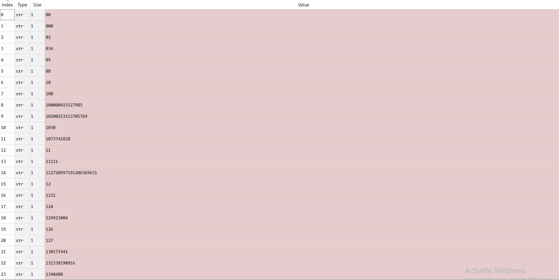
The result found after vectorizing is it starts with numbers and ends with regular words.
向量化后发现的结果是,它以数字开头,以规则的单词结尾。
Shuffling the dataset
改组数据集
The following command shuffles the dataset with fraction 100% that is adding frac=1:
以下命令将分数添加为frac = 1的分数为100%的数据进行混洗:
dshuf = df.sample(frac = 1)Splitting the Dataset
分割数据集
We will split the dataset into training and testing sets. Let’s assume that the first 300 will be for training, while the latter 50 will be for testing:
我们将数据集分为训练和测试集。 假设前300个用于培训,而后50个用于测试:
dtrain = dshuf[:300]
dtest = dshuf[300:]
dtrain_att = vectorizer.fit_transform(dtrain[‘CONTENT’])
dtest_att = vectorizer.transform(dtest[‘CONTENT’])
dtrain_label = dtrain[‘CLASS’]
dtest_label = dtest[‘CLASS’]
In the preceding code, ‘vectorizer.fit_transform(dtrain[‘CONTENT’])’ is an important step. At that stage, you have a training set that you want to perform a fit transform on, which means it will learn the words and also produce the matrix. However, for the testing set, we don’t perform a fit transform again, since we don’t want the model to learn different words for the testing data
在前面的代码中,' vectorizer.fit_transform(dtrain ['CONTENT']) '是重要的一步。 在那个阶段,您有一个训练集,您想对它进行拟合变换,这意味着它将学习单词并生成矩阵。 但是,对于测试集,我们不再执行拟合变换,因为我们不希望模型为测试数据学习不同的词
Building the Random Forest Classifier
建立随机森林分类器
We will begin with the building of the random forest classifier. We will be converting this dataset into 80 different trees and we will fit the training set so that we can score its performance on the testing set:
我们将从构建随机森林分类器开始。 我们将把这个数据集转换成80棵不同的树,我们将拟合训练集,以便我们可以在测试集上对它的性能进行评分:
from sklearn.ensemble import RandomForestClassifier
RFC = RandomForestClassifier(n_estimators = 80, random_state = 0)
RFC.fit(dtrain_att, dtrain_label)
RFC.score(dtrain_att, dtrain_label)
The output of the score is 97.33%, That’s a really good score.
分数的输出是97.33%,这是一个非常好的分数。
Performing a Confusion matrix to check for the number of correct responses:
执行混淆矩阵以检查正确响应的数量:
from sklearn.metrics import confusion_matrix
y_pred = RFC.predict(dtrain_att)
confusion_matrix(y_pred, dtrain_label)
As you can see, we have a total of 292 correct predictions out of 300, That’s a prety good accuracy.
如您所见,在300个样本中,我们总共有292个正确的预测,这是非常好的准确性。
We need be sure that the accuracy remains high ; for that, we will perform a cross validation with five different splits.
我们需要确保准确性很高; 为此,我们将使用五个不同的分割进行交叉验证。
Cross-Validation
交叉验证
To perform a cross validation, we will use all the training data and let it split it into four different groups: 20%, 80%, and 20% will be testing data, and 80% will be the training data:
为了执行交叉验证,我们将使用所有训练数据并将其分为四个不同的组:20%,80%和20%将是测试数据,而80%将是训练数据:
from sklearn.model_selection import cross_val_score
scores = cross_val_score(RFC, dtrain_att, dtrain_label, cv=5)
scores.mean()
After performing an average to the scores that we just obtained, we receive an accuracy of 88.66%.
在对我们刚获得的分数进行平均后,我们获得了88.66%的准确性。
Loading all the datasets
加载所有数据集
Now, we will load all the datasets & combine them
现在,我们将加载所有数据集并将其合并
df = pd.concat([pd.read_csv(‘D:\\Machine Learning_Algoritms\\Youtube-Spam-Check\\Youtube01-Psy.csv’, encoding =’latin1'), pd.read_csv(‘D:\\Machine Learning_Algoritms\\Youtube-Spam-Check\\Youtube02-KatyPerry.csv’, encoding =’latin1'), pd.read_csv(‘D:\\Machine Learning_Algoritms\\Youtube-Spam-Check\\Youtube03-LMFAO.csv’, encoding =’latin1'), pd.read_csv(‘D:\\Machine Learning_Algoritms\\Youtube-Spam-Check\\Youtube04-Eminem.csv’, encoding =’latin1'), pd.read_csv(‘D:\\Machine Learning_Algoritms\\Youtube-Spam-Check\\Youtube05-Shakira.csv’, encoding =’latin1')])The entire dataset has five different videos with comments, which means all together we have around 2,000 rows. On checking all the comments, we noticed that there are 1005 spam comments and 951 not-spam comments, that quite close enough to split it in to even parts:
整个数据集有五个不同的带注释的视频,这意味着我们总共约有2,000行。 在检查所有评论时,我们注意到有1005个垃圾评论和951个非垃圾评论,它们之间的距离足够近,足以将其分成几部分:
df[‘CLASS’].value_counts()
Further, we will shuffle the entire dataset and separate the comments and the answers:
此外,我们将重新整理整个数据集,并将注释和答案分开:
dshuf = df.sample(frac=1)
d_content = dshuf[‘CONTENT’]
d_label = dshuf[‘CLASS’]
We need to perform a couple of steps here with ‘CountVectorizer’ followed by the random forest. For this, we will use a feature in scikit-learn called a Pipeline. Pipeline is really convenient and will bring together two or more steps so that all the steps are treated as one. So, we will build a pipeline with the bag of words, and then use ‘CountVectorizer’ followed by the random forest classifier. Then we will print the pipeline, and it the steps required:
我们需要在此处执行“ CountVectorizer ”和随机森林之后的几个步骤。 为此,我们将使用scikit-learn中的一项名为Pipeline的功能。 流水线确实很方便,它将两个或多个步骤组合在一起,因此所有步骤都被视为一个步骤。 因此,我们将使用一堆单词来构建管道,然后使用“ CountVectorizer ”和随机森林分类器。 然后,我们将打印管道,并执行所需的步骤:
from sklearn.pipeline import Pipeline,make_pipeline
pl = Pipeline([
 (‘bag of words: ‘, CountVectorizer()),
 (‘Random Forest Classifier:’, RandomForestClassifier())])make_pipeline(CountVectorizer(), RandomForestClassifier())
We can let the pipeline name of each step by itself by adding ‘CountVectorizer’ in our ‘RandomForestClassifier’ and it will name them ‘countvectorizer’ and ‘randomforestclassifier’
我们可以通过我们的“RandomForestClassifier”添加“CountVectorizer”本身让每一步的管道名称,它将它们命名为“countvectorizer”和“randomforestclassifier”
Once the pipeline is created you can just call it fit and it will perform the rest that is first it perform the fit and then transform with the ‘CountVectorizer’, followed by a fit with the ‘RandomForestClassifier’ classifier. That’s the benefit of having a pipeline:
一旦创建了管道,您就可以称其为fit,它将执行其余的工作,首先执行拟合,然后使用CountVectorizer进行转换,然后使用RandomForestClassifier分类器进行拟合。 拥有管道的好处是:
pl.fit(d_content[:1500],d_label[:1500])Now you call score so that it knows that when we are scoring it will to run it through the bag of words ‘CountVectorizer’, followed by predicting with the ‘RandomForestClassifier’:
现在,您呼叫分数,以便它知道,当我们进球它将通过话“CountVectorizer”,然后用“RandomForestClassifier”预测的包运行它:
pl.score(d_content[:1500],d_label[:1500])
This whole procedure will produce a score of about 98.3%. We can only predict a single example with the pipeline. For example, imagine we have a new comment after the dataset has been trained, and we want to know whether the user has just typed this comment or whether it’s spam:
整个过程将产生大约98.3%的分数。 我们只能用管道预测一个例子。 例如,假设在训练了数据集之后我们有一个新注释,并且我们想知道用户是否刚刚键入了此注释或它是否是垃圾邮件:
pl.predict([“What a nice video”])
As you can see, it has detected correctly.
如您所见,它已正确检测到。
pl.predict([“Plz subscribe my channel”])
We will use our pipeline to figure out how accurate our cross-validation was:
我们将使用管道来确定交叉验证的准确性:
scores = cross_val_score(pl, d_content, d_label, cv=5)
scores.mean()
In this case, we find that the average accuracy was about 89.3%It’s pretty good. Now let’s add TF-IDF to our model to make it more precise.
在这种情况下,我们发现平均准确度约为89.3%。 现在,将TF-IDF添加到我们的模型中以使其更加精确。
If you are not familiar with TF-IDF is, here is a brief description about it:
如果您不熟悉TF-IDF,这里是对此的简要说明:
TF-IDF
特遣部队
The TfidfVectorizer is a feature that will tokenize documents, learn the vocabulary and inverse document frequency weightings, and allow you to encode new documents.Its primary function is to evaluate how relevant a word is to a document in a collection of documents, which is done by multiplying two metrics: how many times a word appears in a document, and the inverse document frequency of the word across a set of documents.
TfidfVectorizer是一项功能,它将标记文档,学习词汇和逆文档频率加权,并允许您对新文档进行编码。它的主要功能是评估单词与文档集合中的文档的相关性。将两个指标相乘:一个单词在文档中出现的次数,以及单词在一组文档中的反文档频率。
Adding TF-IDF to our model:
将TF-IDF添加到我们的模型中:
from sklearn.feature_extraction.text import TfidfTransformer
pl_2 = make_pipeline(CountVectorizer(), TfidfTransformer(norm=None),
 RandomForestClassifier())
This will be placed after ‘CountVectorizer’. After we have produced the counts, we can then produce a TF-IDF score for these counts. Now we will add this in the pipeline and perform another cross-validation check with the same accuracy:
这将放置在“ CountVectorizer ”之后。 产生计数后,我们可以为这些计数产生TF-IDF分数。 现在,我们将其添加到管道中,并以相同的精度执行另一个交叉验证检查:
scores = cross_val_score(pl_2, d_content, d_label, cv=5)
scores.mean()
On adding TF-IDF, we receive an accuracy of 95.6% for our model.
添加TF-IDF后,我们模型的准确性为95.6%。
There’s another feature of scikit-learn available that allows us to search all of the parameters and then it finds out what the best parameters are:
scikit-learn的另一个功能可用,它使我们可以搜索所有参数,然后找出最佳参数:
parameters = {
 ‘countvectorizer__max_features’: (1000, 2000),
 ‘countvectorizer__ngram_range’: ((1, 1), (1, 2)),
 ‘countvectorizer__stop_words’: (‘english’, None),
 ‘tfidftransformer__use_idf’: (True, False),
 ‘randomforestclassifier__n_estimators’: (10, 30, 50)
 }
We can make a little dictionary where we say the name of the pipeline step and then mention what the parameter name would be and this gives us our options. For demonstration, we are going to try maximum number of words or maybe just a maximum of 1,000 or 2,000 words. Using ‘ngrams’, we can mention just single words or pairs of words that are stop words, use the English dictionary of stop words, or don’t use stop words, which means in the first case we need to get rid of common words, and in the second case we do not get rid of common words. Using TF-IDF, we use JEG to state whether it’s yes or no. The random forest we created uses 20, 50, or 100 trees. Using this, we can perform a grid search, which runs through all of the combinations of parameters and finds out what the best combination is. So, let’s give our pipeline number 2, which has the TF-IDF along with it.
我们可以制作一个小词典,在其中说出管道步骤的名称,然后提及参数名称将是什么,这为我们提供了选择。 为了演示,我们将尝试最大单词数,或者最多尝试1,000或2,000个单词。 使用“ ngrams”,我们可以仅提及单个单词或成对的单词作为停用词,使用停用词的英语词典,或者不使用停用词,这意味着在第一种情况下,我们需要摆脱常用词,在第二种情况下,我们不会摆脱常见的单词。 使用TF-IDF,我们使用JEG声明是或否。 我们创建的随机森林使用20、50或100棵树。 使用此工具,我们可以执行网格搜索,遍历所有参数组合并找出最佳组合。 因此,让我们给我们的管道编号2加上TF-IDF。
To Check the list of available parameters in grid_search:
要检查grid_search中的可用参数列表:
grid_search.estimator.get_params()We will use ‘fit’ to perform the search:
我们将使用“适合”来执行搜索:
grid_search.fit(d_content, d_label)
Since there is a large number of words, it takes a little while, around 50 seconds (in my case) , and ultimately finds the best parameters. We can get the best parameters out of the grid search and print them to see what the score is:
由于存在大量单词,因此需要花费一些时间(大约50秒)(对于我而言),最终找到最佳参数。 我们可以从网格搜索中获得最佳参数,并打印它们以查看分数:
print(“Best accuracy:” , grid_search.best_score_)
print(“Best parameters: “)
best_params = grid_search.best_estimator_.get_params()
for name in sorted(best_params.keys()):
   print(‘{} : {}’.format(name, best_params[name]))
So, we got nearly 96% accuracy. We used around 1,000 words, only single words, used yes to get rid of stop words, had 30 trees in the random forest, and used yes and the IDF and the TF-IDF computation. Here we’ve demonstrated not only bag of words, TF-IDF, and random forest, but also the pipeline feature and the parameter search feature known as grid search.
因此,我们获得了近96%的准确性。 我们使用了大约1,000个单词,只有一个单词,使用yes摆脱了停用词,在随机森林中有30棵树,并使用yes和IDF和TF-IDF计算。 在这里,我们不仅展示了单词袋,TF-IDF和随机森林,还展示了管道功能和称为网格搜索的参数搜索功能。
If you want to look at my other projects, here is the GitHub repository:https://github.com/AkshayLaddha943
如果要查看我的其他项目,请访问GitHub存储库: https : //github.com/AkshayLaddha943
翻译自: https://medium.com/@akshmahesh/detecting-spam-comments-on-youtube-using-machine-learning-948d54f47b3


 436
436

 被折叠的 条评论
为什么被折叠?
被折叠的 条评论
为什么被折叠?
 到【灌水乐园】发言


