双阈值检测阈值选择
In my earlier post, I talked about finding lane lines using Edge Detection and Hough Transforms. While Canny edge detection is great in finding the edges, it gives you a lot of edges in the picture, all of which are not relevant for the lane finding.
在我以前的文章中,我谈到了使用“边缘检测”和“霍夫变换”来查找车道线。 尽管Canny边缘检测可以很好地发现边缘,但它可以为您提供图片中的许多边缘,而所有这些边缘都不与车道发现相关。
In this post, I would describe how to create a pipeline to find lane markings from a video using better algorithms than the last post. The pipeline would mark the lane, project the marked lane onto the video, tell the curvature of the road and also the position of the vehicle within that lane. I would use some of the concepts that I described before like camera calibration, perspective transform as well as a few new ones like thresholding, sliding window etc.
在这篇文章中,我将介绍如何使用比上一篇文章更好的算法创建管道以从视频中查找车道标记。 管道将标记车道,将标记的车道投影到视频上,告知道路的曲率以及车辆在该车道内的位置。 我将使用我之前介绍的一些概念,例如相机校准,透视变换以及一些新概念,例如阈值,滑动窗口等。
To begin with, the images were corrected for camera distortion using the algorithm described in my previous post. The next task was to identify the pixels in picture that belongs to the lane markings for which I used Gradient and Colour Thresholding.
首先,使用我之前的文章中描述的算法对图像进行相机失真校正。 下一个任务是识别图片中属于车道标记的像素,为此我使用了“渐变”和“颜色阈值”。
梯度阈值 (Gradient Threshold)
In the Canny Edge Detection, we took the overall gradient which helped us in detecting the regions which had sharp change in intensity or colour. For this ,canny edge detection uses Sobel operator which is an approximation to taking a derivative of image in a direction. The operator consists of a pair of convolution kernels.
在Canny Edge Detection中,我们采用了整体梯度,这有助于我们检测强度或颜色急剧变化的区域。 为此,canny边缘检测使用Sobel算子,该算子近似于沿方向获取图像的导数。 运算符由一对卷积内核组成。

The magnitude of overall gradient is given by the formula:
总梯度的大小由以下公式给出:

While the direction of the gradient is
而渐变的方向是

Instead of taking overall gradient let’s try to separate out magnitude and Direction of Gradient. This can provide greater advantages in some cases. Lane lines, if the lanes are not too curved, in an image would be close to vertical. So a x direction gradient would make more sense than a y direction. Taking individual x and y gradients or taking the magnitude of the gradient or just taking the direction of the gradient can all have their advantages. We can apply different thresholding on each to arrive at a desired outcome.
让我们尝试分离出幅度和梯度方向,而不是采用整体梯度。 在某些情况下,这可以提供更大的优势。 车道线,如果车道不太弯曲,则图像中的垂直线将接近。 因此,ax方向梯度比ay方向更有意义。 采用单独的x和y梯度或采用梯度的大小或仅采用梯度的方向都具有其优点。 我们可以对每个应用不同的阈值以达到期望的结果。
Sobel X, Y threshold
Sobel X,Y阈值
OpenCV has a sobel function to take the gradient in x,y direction which can be used to also create magnitude and direction only thresholds using the formula above. It is not exactly necessary to convert your figure to grayscale but it provides better visuals. Thresholding is just a way to create a binary image where every pixel that meets the condition is changed to 1 and other pixels are set to 0.
OpenCV具有sobel函数,可沿x,y方向获取梯度,该函数还可用于使用上述公式创建仅幅度和方向的阈值。 完全不需要将图形转换为灰度,但可以提供更好的视觉效果。 阈值只是创建二进制图像的一种方法,其中将满足条件的每个像素更改为1,将其他像素设置为0。
import numpy as np
import cv2
import matplotlib.pyplot as plt
import matplotlib.image as mpimg
import pickle# Read in an image and grayscale it
image = mpimg.imread('straight_lines1.jpg')# Define a function that applies Sobel x or y,
# then takes an absolute value and applies a threshold.
# Note: calling your function with orient='x', thresh_min=5, thresh_max=100
def abs_sobel_thresh(img, orient='x', thresh_min=0, thresh_max=255):
    # Apply the following steps to img    # 1) Convert to grayscale
    gray = cv2.cvtColor(img, cv2.COLOR_RGB2GRAY)    # 2) Take the derivative in x or y given orient = 'x' or 'y'
    sobel = cv2.Sobel(gray, cv2.CV_64F, orient=='x', orient=='y')    # 3) Take the absolute value of the derivative or gradient
    abs_sobel = np.absolute(sobel)    # 4) Scale to 8-bit (0 - 255) then convert to type = np.uint8
    scaled_sobel = np.uint8(255*abs_sobel/np.max(abs_sobel))    # 5) Create a mask of 1's where the scaled gradient magnitude
            # is > thresh_min and < thresh_max
    sxbinary = np.zeros_like(scaled_sobel)
    sxbinary[(scaled_sobel >= thresh_min) & (scaled_sobel <= thresh_max)] = 1# 6) Return this mask as your binary_output image
    binary_output = sxbinary # Remove this line
    return binary_output
# Run the functiongrad_binary_x = abs_sobel_thresh(image, orient='x', thresh_min=20, thresh_max=100)grad_binary_y = abs_sobel_thresh(image, orient='y', thresh_min=20, thresh_max=100)# Plot the result
f, (ax1, ax2, ax3) = plt.subplots(1, 3, figsize=(24, 9))
f.tight_layout()
ax1.imshow(image)
ax1.set_title('Original Image', fontsize=30)
ax2.imshow(grad_binary_x, cmap='gray')
ax2.set_title('Thresholded Gradient in X', fontsize=30)
ax3.imshow(grad_binary_y, cmap='gray')
ax3.set_title('Thresholded Gradient in Y', fontsize=30)
plt.subplots_adjust(left=0., right=1, top=0.9, bottom=0.)
The output of the code above shows the differences between different thresholding. Notice how X gradient thresholding seems a bit better to suit our needs here.
上面代码的输出显示了不同阈值之间的差异。 请注意,X梯度阈值处理似乎更好地适合了我们的需求。

Similarly using the Magnitude of the overall gradient as the threshold can combine some of the individual X, Y gradient features.
类似地,使用整体梯度的幅值作为阈值可以组合一些单独的X,Y梯度特征。

Similarly we can apply threshold on direction of the gradient. As you can see the lane lines are somewhere in 45 to 60 degree range in these figures. Appropriate tan values could be used cover that angle range.
同样,我们可以在梯度方向上应用阈值。 如您所见,这些图中的车道线在45至60度范围内。 可以在该角度范围内使用适当的正切值。

色彩空间 (Colour Spaces)
Colour spaces are very useful tool to analyse images. There are various colour space models that can be used to define the colours in an image. The simplest RGB (Red Green Blue) model defines colours in terms of their red, green, and blue components. Each component can take a value between 0 and 255, where [0,0,0] represents black and [255,255,255] represents white. RGB is considered an “additive” color space and colors can be imagined as different combinations of red, green and blue. OpenCV has multiple functions to utilise different colourspaces. One more thing to note though is that OpenCV by default reads an image in BGR which can be converted to RGB.
色彩空间是分析图像的非常有用的工具。 有多种颜色空间模型可用于定义图像中的颜色。 最简单的RGB(红色绿色蓝色)模型根据红色,绿色和蓝色成分定义颜色。 每个分量可以取0到255之间的值,其中[0,0,0]代表黑色,[255,255,255]代表白色。 RGB被认为是“加法”颜色空间,可以将颜色想象成红色,绿色和蓝色的不同组合。 OpenCV具有多种功能来利用不同的色彩空间。 不过要注意的另一件事是,OpenCV默认会读取BGR中的图像,该图像可以转换为RGB。

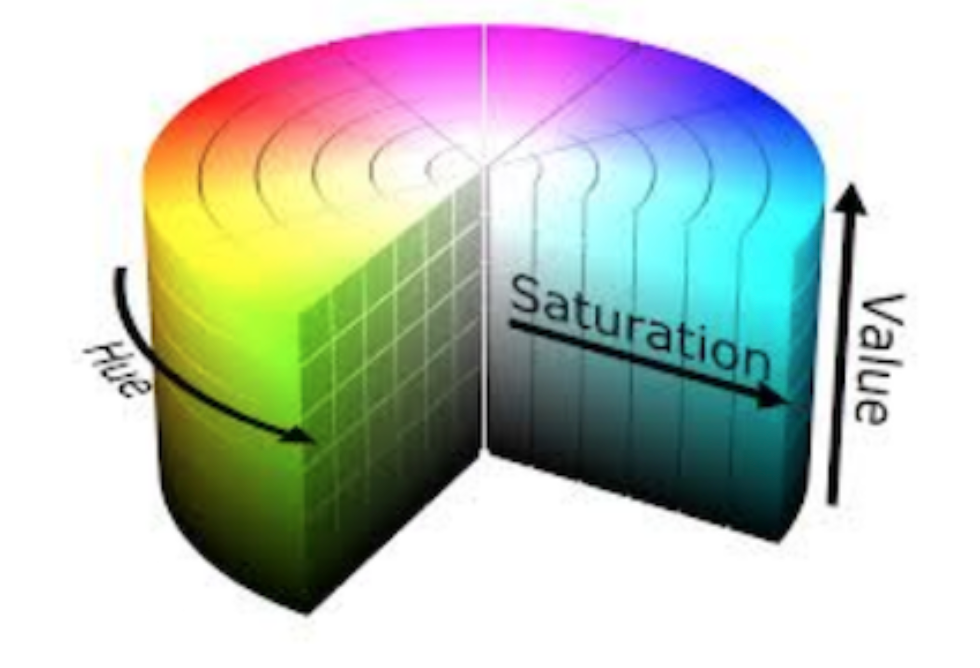
Notice how in blue channel, yellow lane lines are not visible while they are brightest in the Red channel. So here Red channel can be the most useful one to find lane lines. Please note that I have used a greyscale map to show different colour channels. Apart from RGB, there are multiple other colour space models like CMYK, HLS, HSV, LAB etc. HSV and HLS stands for hue, saturation, and brightness/luminance, which are particularly useful for identifying contrast in images.
请注意,在蓝色通道中,黄色车道线在红色通道中最亮时却不可见。 因此,这里红色通道可能是查找车道线最有用的通道。 请注意,我使用了灰度图来显示不同的颜色通道。 除RGB外,还有其他多种颜色空间模型,例如CMYK,HLS,HSV,LAB等。HSV和HLS 代表色相,饱和度和亮度/亮度,它们对于识别图像的对比度特别有用。

Hue is the different colours, Saturation is how intense the colour is and value is the brightness value. You can try out different colourspace and colour channels to see what works for your application. Once you know the correct colourspace and colour channel, you can apply thresholding. For my purpose I found the S channel in HLS colourspace to be the best suited.
色相是不同的颜色,饱和度是颜色的强烈程度,值是亮度值。 您可以尝试不同的色彩空间和颜色通道,以查看适合您的应用程序的颜色。 一旦知道正确的色彩空间和色彩通道,就可以应用阈值设置。 出于我的目的,我发现最适合HLS色彩空间中的S通道。

I applied colour thresholding on that using the following code:
我使用以下代码对此应用了颜色阈值:
import matplotlib.pyplot as plt
import matplotlib.image as mpimg
import numpy as np
import cv2# Read in an image, you can also try test1.jpg or test4.jpg
image = mpimg.imread('straight_lines1.jpg')# Define a function that thresholds the S-channel of HLS
# Use exclusive lower bound (>) and inclusive upper (<=)
def hls_select(img, thresh=(0, 255)):
    # 1) Convert to HLS color space
    hls = cv2.cvtColor(img, cv2.COLOR_RGB2HLS)
    # 2) Apply a threshold to the S channel
    binary_output = np.zeros_like(hls[:,:,2])
    binary_output[(hls[:,:,2] > thresh[0]) & (hls[:,:,2] <= thresh[1])] = 1
    # 3) Return a binary image of threshold result
    #binary_output = np.copy(img) # placeholder line
    return binary_output
hls_binary = hls_select(image, thresh=(180, 255))# Plot the result
f, (ax1, ax2) = plt.subplots(1, 2, figsize=(24, 9))
f.tight_layout()
ax1.imshow(image)
ax1.set_title('Original Image', fontsize=50)
ax2.imshow(hls_binary, cmap='gray')
ax2.set_title('Thresholded S', fontsize=50)
plt.subplots_adjust(left=0., right=1, top=0.9, bottom=0.)
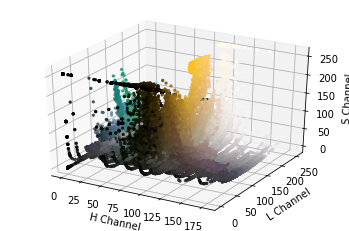
It is not always easy to arrive at the correct thresholding values. One way to do it might be to use 3D scatterplot. We can plot the individual channels for the picture and then approximate the values we might be interested in.
得出正确的阈值并不总是容易的。 一种方法是使用3D散点图。 我们可以绘制图片的各个通道,然后近似我们可能感兴趣的值。

Once you know what gradient, colourspace and channel to use, you can combine the various thresholds. For this particular project, I used X direction gradient along with S- Channel in HLS colourspace to apply the thresholds.
一旦知道要使用的渐变,色彩空间和通道,就可以组合各种阈值。 对于此特定项目,我在HLS色彩空间中使用了X方向梯度和S通道来应用阈值。
Perspective Transform(as described in the previous post) was applied to the resultant binary image to get the birds view. In 2D images, objects appear smaller the farther away they are from a viewpoint. So it is better to perform a perspective transform on the undistorted thresholded image to have a birdeye view of how the lane lines are so that later, the curve fitting through them can be done accurately
透视变换(如先前文章中所述)被应用到生成的二进制图像以获得鸟瞰图。 在2D图像中,对象距视点越远显得越小。 因此,最好对未变形的阈值图像执行透视变换,以鸟瞰车道线,以便以后可以精确地拟合通过它们的曲线

The colours look different in the picture as the matplotlib and opencv reads in images differently( RGB vs BGR). The next step was to fit the curves along the lane lines.
由于matplotlib和opencv读取图像的方式不同(RGB与BGR),因此颜色在图片中看起来也有所不同。 下一步是沿车道线拟合曲线。
线查找方法:直方图中的峰 (Line Finding Method: Peaks in a Histogram)
After applying calibration, thresholding, and a perspective transform to a road image, you should have a binary image where the lane lines stand out clearly. However, you still need to decide explicitly which pixels are part of the lines and which belong to the left line and which belong to the right line. Plotting a histogram of where the binary activations occur across the image is one potential solution for this. Taking a histogram along all the columns in the lower half of the image like this:
在对道路图像应用校准,阈值和透视变换后,您应该拥有一个二进制图像,其中车道线清晰可见。 但是,您仍然需要明确决定哪些像素是线条的一部分,哪些像素属于左线条,哪些像素属于右线条。 对此图像绘制二进制激活在何处发生的直方图是一种可能的解决方案。 直方图 沿着图像下半部分的所有列,如下所示:

The two most prominent peaks in this histogram will be good indicators of the x-position of the base of the lane lines. We can use that as a starting point for where to search for the lines. From that point, we can use a sliding window, placed around the line centers, to find and follow the lines up to the top of the frame.
该直方图中最突出的两个峰将很好地指示车道线底部的x位置。 我们可以将其用作在哪里搜索线的起点。 从这一点开始,我们可以使用围绕线心放置的滑动窗口来查找并跟随线直到框架的顶部。
滑动窗算法 (Sliding window Algorithm)
The following algorithm was followed:
遵循以下算法:
1- All the non-zero pixels are identified in the image
1-在图像中识别所有非零像素
2-Next a sliding window is defined at the x positions of lane and all the non-zero pixels appearing inside the window are identified.
2-接着,在泳道的x位置处定义滑动窗口,并且识别出现在窗口内的所有非零像素。
3- The sliding window is moved in Y direction to find more non zero pixels and offsetted in X to their mean in case we find more than a set number.
3-滑动窗口沿Y方向移动,以找到更多的非零像素,如果发现的数量多于设定数量,则X偏移其平均值。
4- Once we have all the good pixel candidates for lanes in the entire image, a second degree polynomial is fitted through them f(y)=Ay2+By+C
4-一旦我们拥有了整个图像中所有适合泳道的像素候选,就通过它们拟合二阶多项式f(y)= Ay2 + By + C
5- The steps are repeated for left and right lane line separately.
5-分别对左右车道线重复上述步骤。

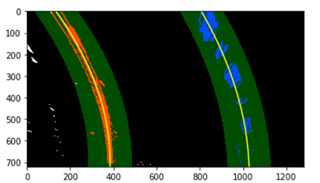
Once you know where the lines are, you have a fit! In the next frame of video, you don’t need to do a blind search again, but instead you can just search in a margin around the previous line position.
一旦知道线条在哪里,就很合适! 在视频的下一帧中,您无需再次进行盲目搜索,而只需在前一行位置周围的空白处搜索即可。

测量曲率 (Measuring Curvature)
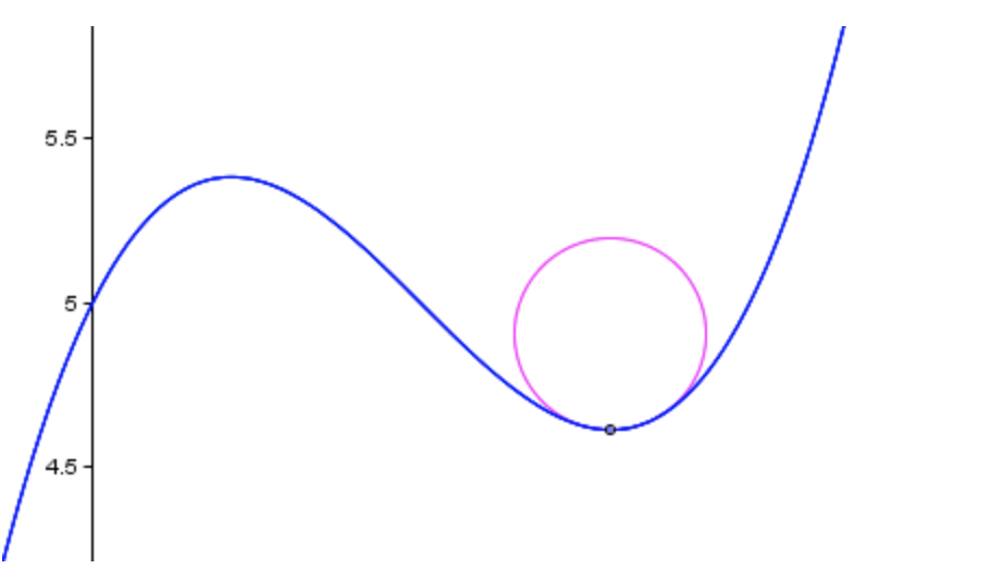
Once the polynomial is fitted through the lane lines, its radius of curvature is calculated using Curvdist() function. We can draw a circle that closely fits nearby points on a local section of a curve.
一旦多项式通过车道线拟合,就可以使用Curvdist()函数计算其曲率半径。 我们可以在曲线的局部区域上绘制一个与附近点非常契合的圆。

The formula for the radius of curvature at any point x for the curve y = f(x) is given by
曲线y = f ( x )的任意点x的曲率半径的公式为

In order to cover the pixel values into the road units the following conversion is used
为了将像素值覆盖到道路单位中,使用以下转换
ym_per_pix = 30/720 xm_per_pix = 3.7/700
ym_per_pix = 30/720 xm_per_pix = 3.7 / 700
where they are in meters per pixel units
它们以米/像素为单位
In order to calculate the distance from the centre, assumption is made that the camera is mounted on the centre of the car. The average of the left and right lane is taken at the bottom of the image and then subtracted from the centre of the image. The distance is then mutiplied by the xm_per_pix to convert it into metres.
为了计算到中心的距离,假设摄像机安装在汽车的中心。 左车道和右车道的平均值在图像的底部获取,然后从图像的中心减去。 然后,将距离乘以xm_per_pix乘以将其转换为米。
Once the lane lines are identified, the full lane is warped back onto the original image using the inverse of the matrix calculated in the perspective transform step.
一旦车道线被识别,就使用在透视变换步骤中计算出的矩阵的逆矩阵将整个车道弯回到原始图像上。
Finally the steps are repeated for every frame to identify the lane lines in the video:
最后,对每一帧重复上述步骤,以识别视频中的车道线:
It marks the lane and the text on the upper left corner tells you the lane curvature and position of the vehicle in that lane.
它标记了车道,左上角的文字告诉您车道的曲率和车辆在该车道中的位置。
This pipeline worked well for the given video. However, it struggled in the cases where lane curvature is more. To solve this, it might be a good idea to store all the coefficients of the fits as a history from frame to frame and look for any significant departures. It might also be useful to update the sliding window to take into account large curvatures.
该管道对于给定的视频效果很好。 但是,在车道曲率更大的情况下,它会遇到困难。 为了解决这个问题,最好将拟合的所有系数存储为一帧到一帧的历史记录,并查找任何重大偏离。 考虑到较大的曲率,更新滑动窗口也可能很有用。
More details and actual code for this project can be found at my github repo
这个项目的更多细节和实际代码可以在我的github仓库中找到
Thanks to Udacity for guiding me through this project.
感谢Udacity指导我完成这个项目。
Written while listening to Fleet Foxes
在听 舰队狐狸时 写的
翻译自: https://medium.com/swlh/computer-vision-advanced-lane-detection-through-thresholding-8a4dea839179
双阈值检测阈值选择


 本文介绍了如何在计算机视觉中通过双阈值检测技术进行高级车道检测,详细阐述了阈值选择的重要性及其在车道检测过程中的应用。


 648
648

 被折叠的 条评论
为什么被折叠?


