


jax-rs jax-ws
TL; DR: Without reliable optimization methods, training ML models is infeasible or too slow to be practically useful. Many of the most powerful optimization methods require calculating loss function derivatives in order to efficiently search the space of possible parameter values. However, computing derivatives of complicated functions is tedious, time-consuming, and prone to human error. Jax is an open-source Python library that provides an automated method for computing derivatives, reducing development cycle time and improving the readability of code.
TL; DR: 没有可靠的优化方法,训练ML模型不可行或太慢而无法实际应用。 许多最强大的优化方法都需要计算损失函数导数,以便有效地搜索可能的参数值的空间。 但是,计算复杂函数的导数是繁琐,耗时的,并且容易发生人为错误。 Jax是一个开放源代码的Python库,它提供了一种自动方法来计算派生类,从而缩短了开发周期并提高了代码的可读性。
ML优化:概述 (Optimization for ML: an overview)
Many machine learning problems can be boiled down to the following steps:
许多机器学习问题可以归结为以下步骤:
- Specify a model with parameters θ that takes in input data and returns a predicted value or set of values. 使用参数θ指定一个模型,该模型可以吸收输入数据并返回预测值或一组值。
- Specify a loss function that captures how dissimilar the predictions of a model are compared to observed “ground truth” data (of course, this is highly problem-dependent). 指定一个损失函数,该函数捕获将模型的预测与观察到的“地面真实”数据进行比较的方式之间的差异(当然,这与问题高度相关)。
- Find the set of parameters θ that minimize the loss function using an optimization routine. 使用优化例程找到使损耗函数最小的参数θ。
Consider the case of linear regression with two independent variables x1 and x2. The model specification is:
考虑具有两个自变量x1和x2的线性回归的情况。 型号规格为:
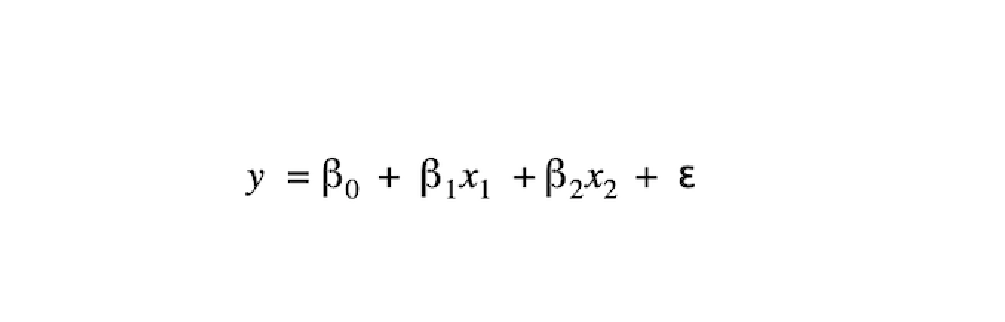
Here, the β values represent the parameters that need to be optimized (taking the place of θ in our more general description above) , ε is an error term that represents uncertainty, and y is the “true” value that we’re trying to predict. The canonical loss function for linear regression is the sum of squared errors:
在此,β值表示需要优化的参数(在上面的更笼统的描述中代替θ),ε是表示不确定性的误差项,而y是我们要尝试的“真实”值预测。 线性回归的规范损失函数是平方误差的总和:
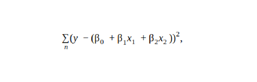
This applies across all of our n data points. Therefore, we’d like to pick the β values such that this value is minimized. In the specific case of linear regression, we can actually solve for the β values analytically using linear algebra. However, in most cases, finding an analytic solution in this way is not possible. Therefore, we turn to optimization methods which allow us to iteratively search for the best parameter values that minimize the loss function for whatever problem we’re trying to solve.
这适用于我们所有n个数据点。 因此,我们希望选择β值以使该值最小。 在线性回归的特定情况下,我们实际上可以使用线性代数解析地求解β值。 但是,在大多数情况下,不可能以这种方式找到分析解决方案。 因此,我们转向优化方法,该方法允许我们迭代地搜索最佳参数值,以针对要解决的任何问题最小化损失函数。
我们为什么需要衍生品? (Why do we need derivatives?)
The space of possible parameter values is usually infinite, so we need a clever way to search for the optimal parameters. Consider the analogy of a blind person lost in the hills who wants to get back to the valley where they parked their car. (Imagine the hills are completely smooth and there are no obstacles to contend with). At each point, they can sense the slope of the hill, and so they proceed by walking downhill, re-calibrating every so often to figure out the direction of the steepest downwards descent and then walking in that direction.
可能的参数值的空间通常是无限的,因此我们需要一种巧妙的方法来搜索最佳参数。 考虑一个在山上迷路的盲人的比喻,他们想回到停放汽车的山谷。 (想象一下,山丘是完全平坦的,没有障碍可争)。 在每个点上,他们都能感觉到山坡,因此,他们走下坡路,经常进行重新校准,以找出最陡峭的下降方向,然后沿着该方向走。
In this analogy, the person’s elevation corresponds to the loss function they want to minimize, and the x and y coordinates of the direction they walk in represent the two parameters of this “model”. This is the essence of many iterative derivative-based optimization methods: by understanding the topography of the region in parameter space, one can determine the direction that most quickly decreases the loss function and hopefully reach the global minimum most quickly.
以此类推,人的高程对应于他们要最小化的损失函数,而他们走入方向的x和y坐标表示此“模型”的两个参数。 这是许多基于迭代导数的优化方法的本质:通过了解参数空间中区域的地形,可以确定最Swift减少损失函数并有望最快达到全局最小值的方向。
Jax如何提供帮助? (How can Jax help?)
For many machine learning models, calculating derivatives of loss functions by hand is downright painful. Online tools such Wolfram Alpha can help accelerate this process, but they still require the user to write Python code to encode the derivative correctly. This isn’t so hard for scalar data inputs, but in practice many machine learning models take vectors or matrices as input, and one incorrectly applied dot product or summation can lead to an incorrect derivative that will crash the optimization routine. If only there was a way to get the computer to do all of this hard work for you….
对于许多机器学习模型,手工计算损失函数的导数是非常痛苦的。 诸如Wolfram Alpha之类的在线工具可以帮助加快这一过程,但是它们仍然需要用户编写Python代码来正确编码衍生代码。 对于标量数据输入来说,这并不难,但是在实践中,许多机器学习模型都将矢量或矩阵作为输入,并且一个错误应用的点积或求和会导致不正确的导数,从而使优化例程崩溃。 如果只有一种方法可以让计算机为您完成所有这些艰苦的工作……。
Enter Jax, an open-source library created by Google that can automatically compute derivatives of native Python and NumPy¹ functions. This means that as a user, you can write numerical functions in Python and use Jax to automatically compute derivatives (including higher-order derivatives!) and use them as input to optimization routines.
输入Jax,这是Google创建的开放源代码库,可以自动计算本机Python和NumPy¹函数的派生类。 这意味着作为用户,您可以使用Python编写数值函数并使用Jax自动计算导数(包括高阶导数!),并将其用作优化例程的输入。
Under the hood, Jax makes use of the technique of autodifferentation, a topic that falls squarely outside the scope of this post (this blog post gives a helpful introduction, though). The good news is, you don’t have to understand anything about how autodiff works² in practice to use Jax — you just need to know the basics of how to set up an optimization problem!
在幕后,Jax利用自动区分技术,该主题完全超出了本文的讨论范围(尽管此博客文章提供了有用的介绍)。 好消息是,您实际上不需要了解autodiff的工作方式²,就可以使用Jax —您只需要了解如何设置优化问题的基础即可!
Let’s walk through a real-life example of how Jax can be used to simplify the implementation of a machine learning model.
让我们来看一个真实的示例,该示例说明如何使用Jax简化机器学习模型的实现。
使用Jax将Weibull混合模型拟合到数据 (Using Jax for fitting Weibull mixture models to data)
One of Tagup’s main algorithmic approaches for improving the decision making of asset managers is our time-to-event (TTE) modeling capabilities. Our TTE models use the unified data history of an asset to predict time until certain events occur such as machine failures, preemptive removals, or maintenance actions (for the remainder of this post, we will discuss the specific case of predicting time until failure, commonly known as survival modeling).
Tagup改进资产管理者决策的主要算法方法之一是事件发生时间(TTE)建模功能。 我们的TTE模型使用资产的统一数据历史记录来预测发生某些事件(例如机器故障,抢先拆除或维护操作)之前的时间(在本文的其余部分中,我们将讨论预测直到发生故障的时间的具体情况,通常称为生存建模 )。
Our convex latent variable (CLV) model works by first fitting a parametric distribution to observed asset lifetimes and then using other available data (nameplate data, sensor readings, weather, etc.) to scale that distribution which we refer to as our base hazard. In future posts, we will discuss our approach to time-to-event modeling in detail (this also involves interesting optimization techniques!), but for the purpose of this post, we will focus on the simpler sub-problem of fitting a distribution to observed machine lifetimes.
我们的凸潜变量(CLV)模型的工作方式是首先将参数分布拟合到观察到的资产寿命,然后使用其他可用数据(铭牌数据,传感器读数,天气等)来缩放该分布,这被称为基本危害 。 在以后的文章中,我们将详细讨论事件建模的方法(这也涉及有趣的优化技术!),但是出于这篇文章的目的,我们将关注于将分布拟合到以下更简单的子问题。观察到的机器寿命。
One of the most common distributions used for modeling machine lifetimes is the Weibull distribution, which is a very flexible distribution that is governed by only two parameters. (See our previous post for a brief introduction to survival modeling and an explanation of fitting a Weibull model to data.)
用于建模机器寿命的最常见的分布之一是Weibull分布 ,这是一种非常灵活的分布,仅由两个参数控制。 (有关生存建模的简要介绍和将Weibull模型拟合到数据的说明,请参阅我们的上一篇文章 。)
However, consider a fleet of assets that contains two distinct sub-populations with different means and variances of lifetimes. A simple Weibull model won’t be able to fit this data very well, because the data is really a mixture of multiple distributions. This inspired us to create a tool for fitting Weibull mixture models to data.
但是,请考虑一组资产,其中包含两个不同的子群体,这些子群体具有不同的均值和生命周期方差。 一个简单的Weibull模型将无法很好地拟合此数据,因为该数据实际上是多个分布的混合 。 这激发了我们创造一个将Weibull混合模型拟合到数据的工具。
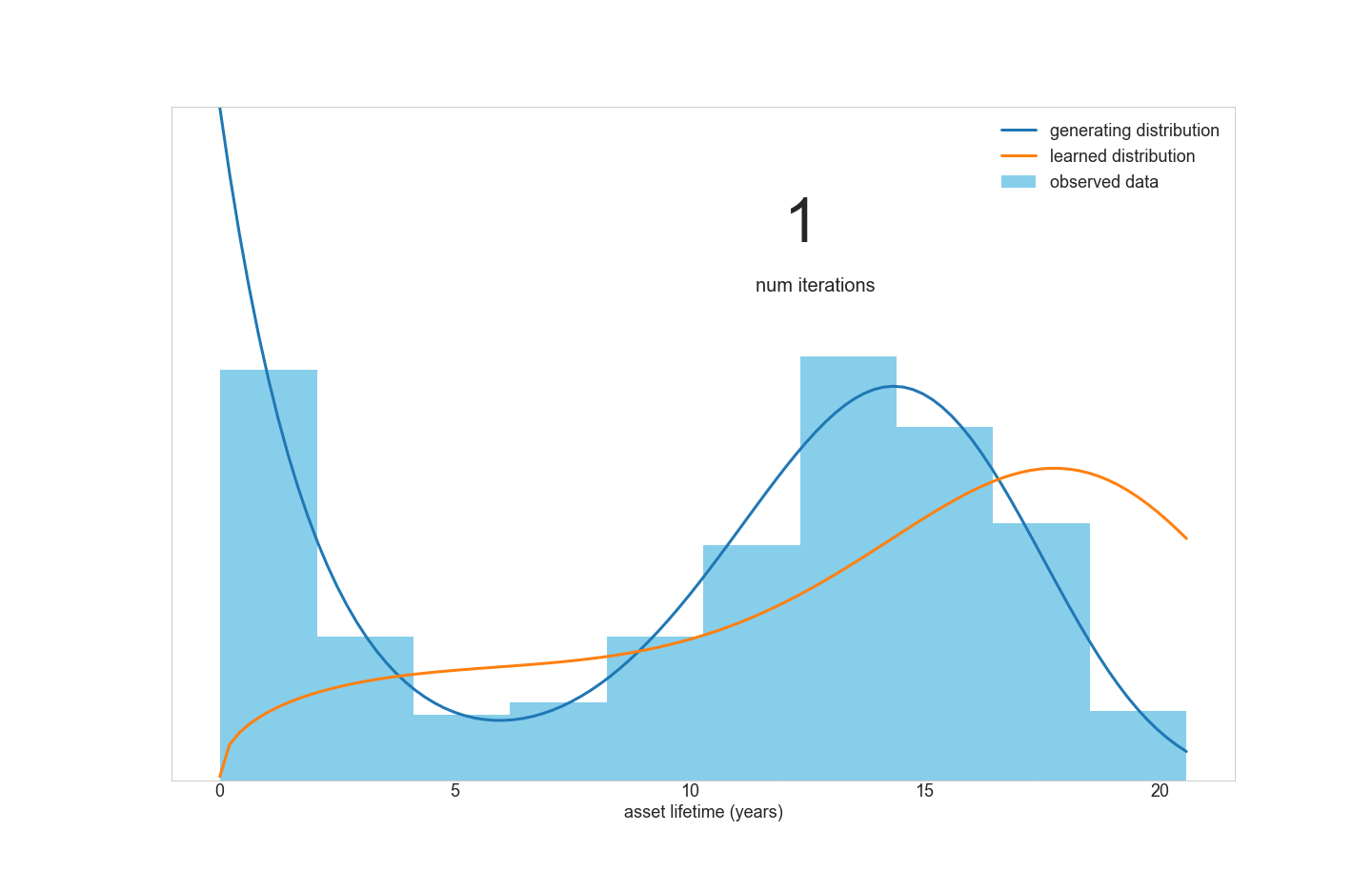
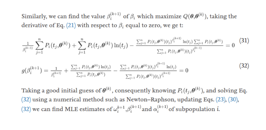
A quick literature review turned up this research paper for doing just that. However, the optimization routine outlined in the paper didn’t look appealing to implement in Python:
快速文献综述使该研究论文得以实现。 但是,本文中概述的优化例程在Python中实现似乎并不吸引人:
How could we avoid the painful process of turning the derivatives into code? The answer, of course, is to use Jax:
我们如何避免将衍生代码转换为代码的痛苦过程? 答案当然是使用Jax:
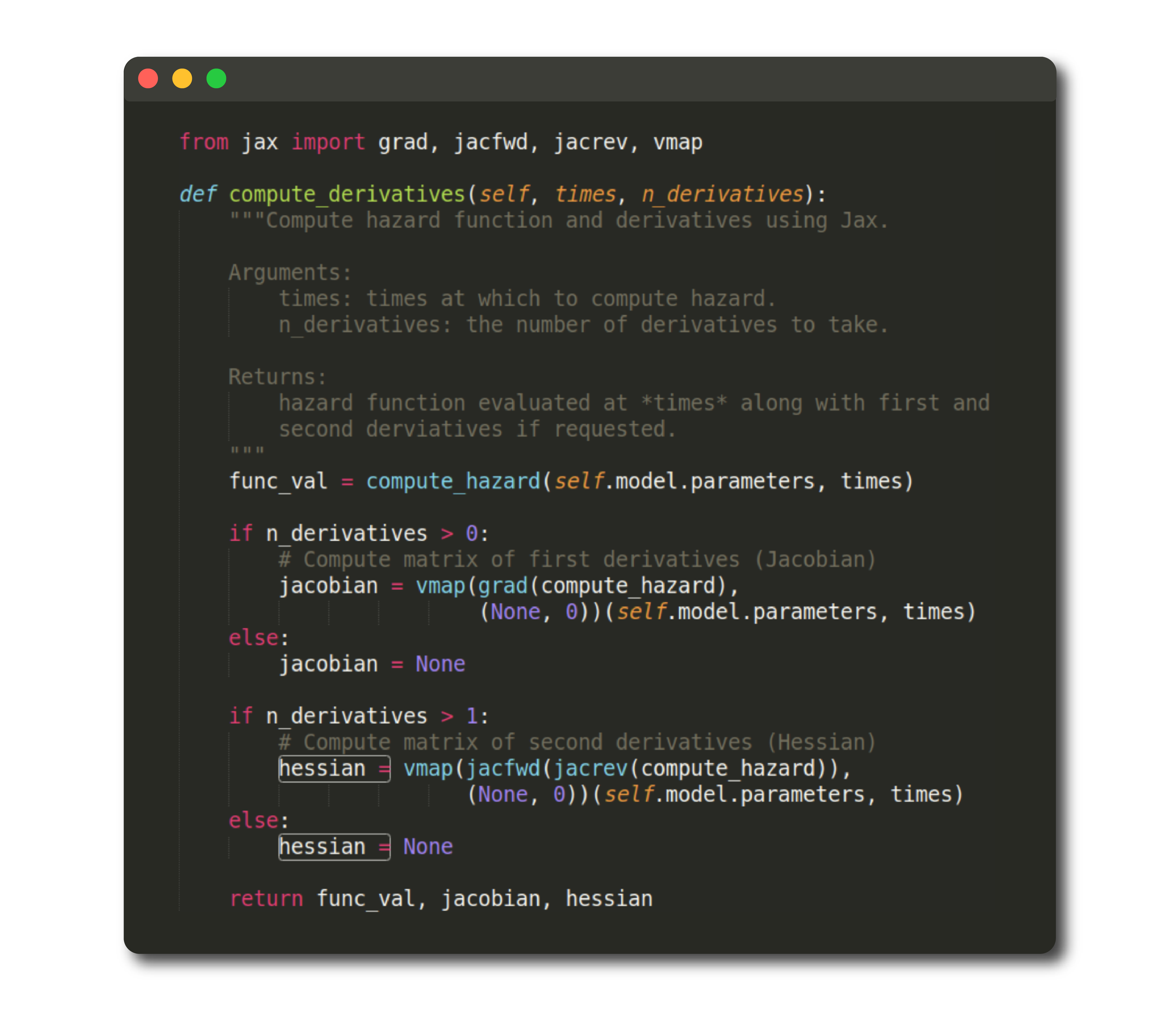
Let’s briefly run through what’s going on in this function, the purpose of which is to compute the hazard³ as a function of model parameters and time since install as well as derivatives of this function if requested.
让我们简要地介绍一下此函数中发生的一切,其目的是根据模型参数和安装以来的时间计算危险³,并根据需要计算该函数的派生形式。
Since compute_hazard is a function of multiple parameters, the derivatives required for optimization are matrices known as the Jacobian (first derivative) and Hessian (second derivative), hence the variable names.
由于compute_hazard是多个参数的函数,因此优化所需的导数是称为Jacobian (一阶导数)和Hessian (二阶导数)的矩阵 ,因此是变量名。
The Jax function grad is used to compute the first derivative of the hazard function, while vmap automatically vectorizes the gradient computation across the inputs (see docs and examples here).
Jax函数grad用于计算危险函数的一阶导数,而vmap自动 对输入中的梯度计算进行矢量化处理(请参阅此处的文档和示例)。
Lastly, jacfwd and jacrev are used in succession to compute the Hessian matrix if requested by the user.
最后,如果用户要求,则连续使用jacfwd和jacrev计算Hessian矩阵。
Wow. In a few simple lines of code, we were able to compute the first and second derivative of the hazard function. Now, all we have to do is pass functions for computing loss and its derivatives to an optimization routine (the specifics of which will be detailed in a future post), and voila, we’re able to find the optimal parameters!
哇。 用几行简单的代码,我们就能计算出危险函数的一阶和二阶导数。 现在,我们要做的就是将计算损失及其导数的函数传递给优化例程(具体细节将在以后的文章中详细介绍),瞧,我们能够找到最佳参数!
结论 (Conclusion)
Optimization is an essential part of making any machine learning problem feasible. Derivative-based optimization methods are by far the most common and reliable approaches used, but require that derivatives be worked out by hand which is often quite tedious and prone to error.
优化是使任何机器学习问题都可行的重要组成部分。 到目前为止,基于导数的优化方法是最常用和最可靠的方法,但是要求手动计算导数,这通常很繁琐并且容易出错。
Jax is an open-source library that seamlessly integrates with Python and uses autodifferentiation to efficiently compute derivatives of complex functions, obviating the need to calculate them manually. It generalizes to many classes of problems common in machine learning and is a very useful tool for data scientists who write custom optimization routines.
Jax是一个开放源代码库,可与Python无缝集成,并使用自动区分功能有效地计算复杂函数的派生,从而无需手动计算它们。 它概括了机器学习中常见的许多类型的问题,并且对于编写自定义优化例程的数据科学家来说是非常有用的工具。
In a future post, we’ll talk more about some considerations and limitations of Jax which will hopefully help you avoid some of the pitfalls we ran into when getting familiar with the library.
在以后的文章中,我们将更多地讨论Jax的一些注意事项和局限性,这些希望和局限性将有助于您避免熟悉图书馆时遇到的一些陷阱。
¹ NumPy is a widely used Python package that provides efficient implementations for numerical computations of the type often required by machine learning models.
¹NumPy是广泛使用的Python软件包,可为机器学习模型经常需要的类型的数值计算提供有效的实现。
² Jax does have some important limitations that users have to be aware of, though — these will be described in a future post.
²不过,Jax确实具有一些用户必须要意识到的重要限制-这些将在以后的文章中进行介绍。
³ In the context of survival modeling, the hazard function represents the probability that an asset fails in period t+1 given that it has lived up until time t. Hazard is convenient to work with for two reasons: the likelihood function that we seek to optimize is a function of hazard; and all statistics of interest (failure probability, expected RUL) can be derived from hazard.
³在生存模型的上下文中, 危害函数 表示资产在t + 1期间发生故障的概率,因为该资产一直存在到t为止。 危害使用起来很方便,原因有两个:我们试图优化的似然函数是危害的函数; 所有关注的统计数据(故障概率,预期RUL)都可以从危害中得出。
jax-rs jax-ws


 1912
1912

 被折叠的 条评论
为什么被折叠?
被折叠的 条评论
为什么被折叠?
 到【灌水乐园】发言


