


python实现代码位于文章底部^~^
3.2数据处理
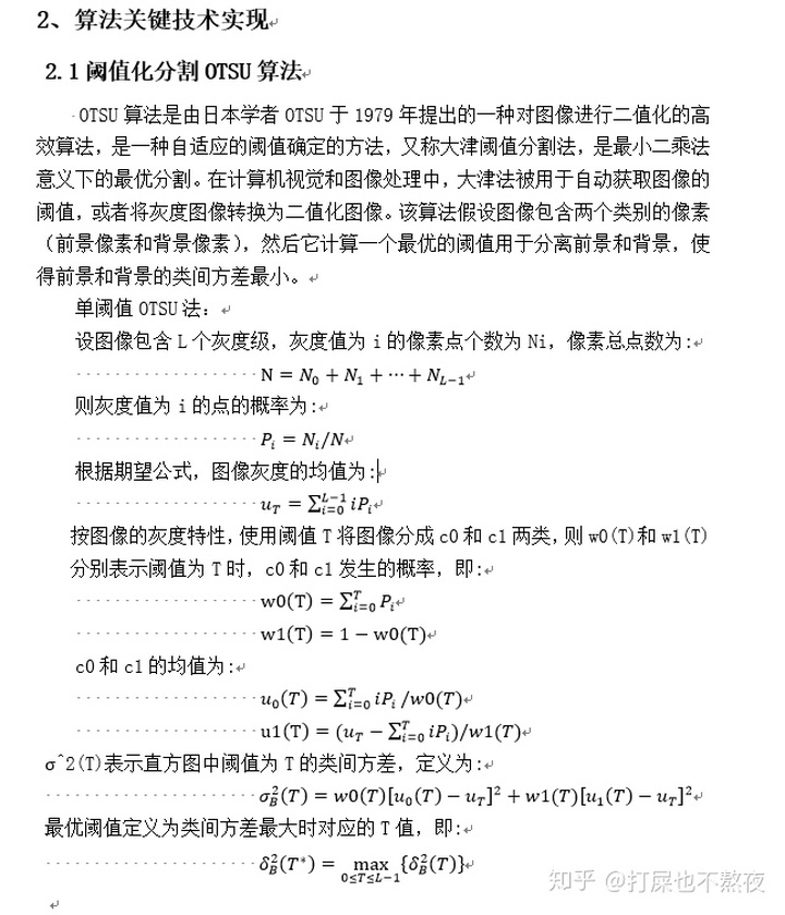
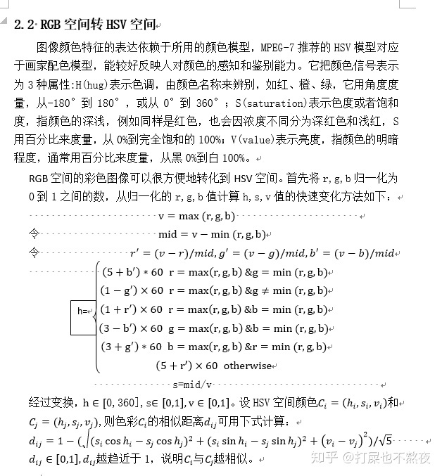
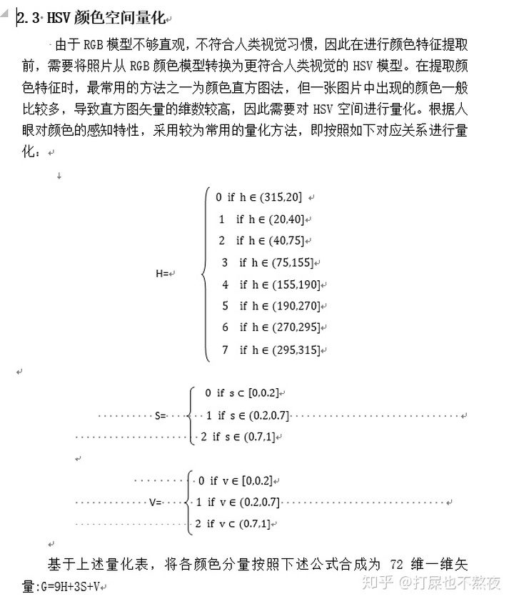
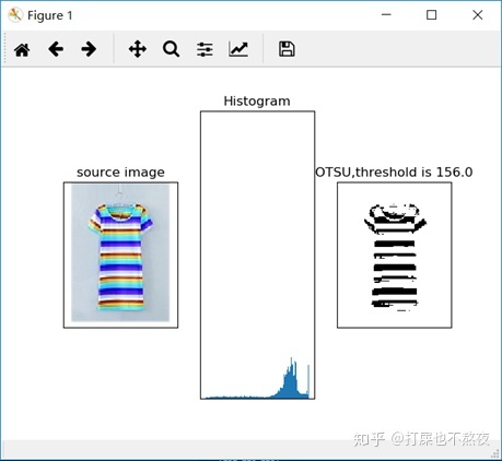
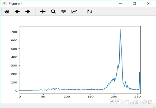
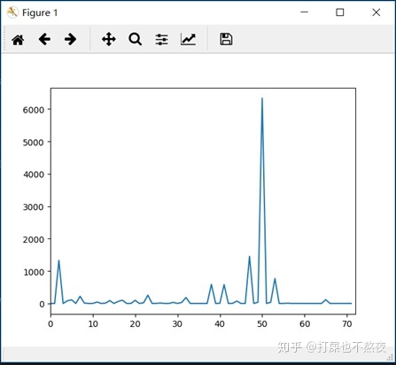
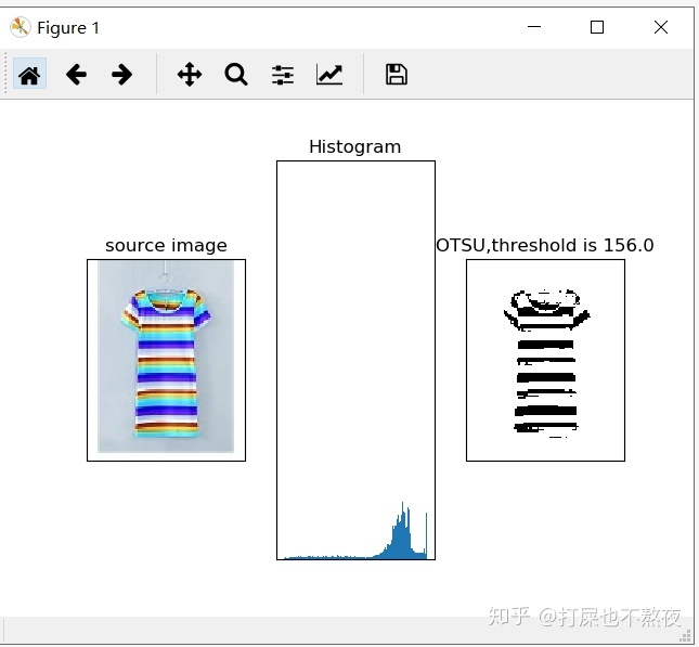
由于本文关注点在于提取服装类图片主题的颜色信息,所以需要先使用OTSU阈值分割算法提取出图像的前景(如图2先算出最优阈值),然后将前景像素矩阵转换成像素点的列表,然后对前景图像进行RGB空间转HSV空间,再进行非等间隔量化处理(如图3和4)。
3.3 对比实验
图5-1,图6-1,图7-1,图8-1为对“整张图像”的色彩进行聚类的结果图,图5-2,图6-2,图7-2,图8-2为只对“前景图像”的色彩进行聚类的结果图。
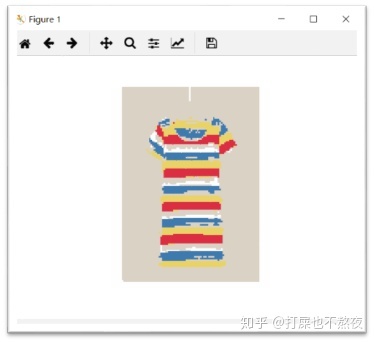
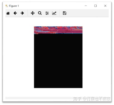
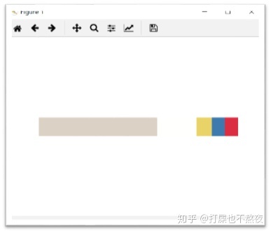
图5-1为对整张图片色彩聚类后并且各个类中的点的像素值被各自聚类中心点的像素值取代后的图像,与原图相比,很明显的看出聚类的效果还是较好的,而图5-2为只对前景衣服主题进行色彩聚类并且各个类中的点的像素值被各自聚类中心点的像素值取代后的图片,由于本算法是将前景中的像素点(坐标及RGB值)抽取出来进行聚类,所以导致图片形状的信息会丢失,所以会出现图5-2所示的图片(看起来已经不是衣服的形状)。
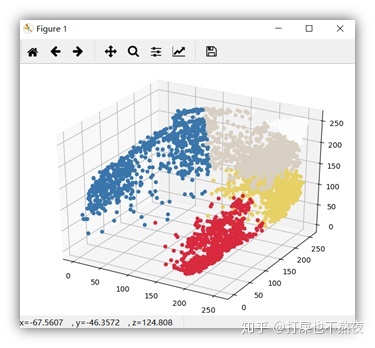
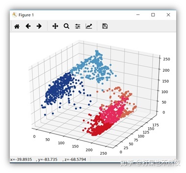
图6-1,图6-2为聚类后,并且各个类中的点的像素值被各自聚类中心点的像素值取代后,将图中各个像素点的立体图可视化,从图中可以看出,同一颜色的点较为明显的聚在一起,而不同颜色的点也较为明显地区分开来。
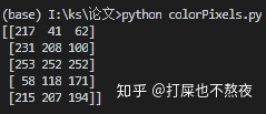
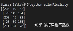
图7-1,图7-2为图像最终得到的聚类中心点集合,可以看出两者之间的差别还是挺大的。
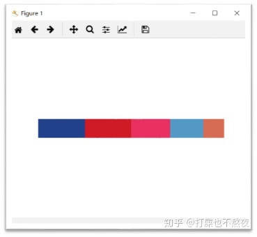
图8-1,图8-2为主要色占比图,可以看出两者之间的色彩种类及色彩占比均不相同。
5、结论与展望
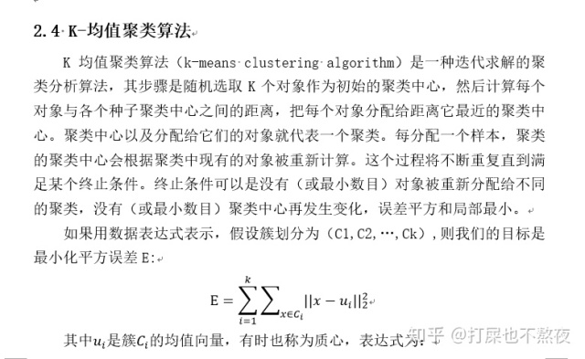
本文采用分割算法得出图像的前景,然后采用K-均值聚类算法对前景进行主颜色提取。实验结果似乎还可以,但是该算法中还存在着问题,比如说采用K-均值聚类时,这个K值不太好确定,有些服装图片中色彩很多,这时如果我们设置的K值过小,则会丢失许多颜色信息,而且每张图片的主体色彩有多少完全没有一致性,所以我们不可能去设置一个统一的K值,所以我们的算法需要在,如何根据图片大体颜色确定一个相应适合的K值这个问题上进行改进,或许我们需要借助深度学习来训练一个模型,该模型能够对输入的每张彩色图片给出一个适合的K值,或者采用KNN,但这两种方法都需要大量打过标签的数据集,而目前还没有公开的这种数据集,所以在使用这个算法时,我们暂时还需要人工根据输入的图像定义一个K值。
由于颜色特征最能体现一件服装的本质特征,也是最稳定的视觉特征,与图像的其他特征相比,具有尺寸、方向、视觉依赖性较小的特点,所以,未来在服装行业有关颜色特征的提取的发展肯定会越来越快,越来越好。
python代码:
#otsu.py  运行该代码实现otsu方法获取分离前后景的最佳像素值
#coding:utf-8
import cv2
import numpy as np
from matplotlib import pyplot as plt

image=cv2.imread("cloth1.jpg")
gray=cv2.cvtColor(image,cv2.COLOR_BGR2GRAY)

plt.subplot(131)
plt.imshow(image,"gray")
plt.title("source image")
plt.xticks([])
plt.yticks([])

plt.subplot(132)
plt.hist(image.ravel(),256)
plt.title("Histogram")
plt.xticks([])
plt.yticks([])

ret1,th1=cv2.threshold(gray,0,255,cv2.THRESH_OTSU)
#方法选择为THRESH_OTSU
plt.subplot(133)
plt.imshow(th1,"gray")
plt.title("OTSU,threshold is "+str(ret1))
plt.xticks([])
plt.yticks([])
plt.show()
运行结果截图:
#dominantColors.py
#一个提取图像主颜色的类,有
# -*- coding: utf-8 -*-


import cv2
import numpy as np
from sklearn.cluster import KMeans
import matplotlib.pyplot as plt
from mpl_toolkits.mplot3d import Axes3D

class DominantColors:

    CLUSTERS = None
    IMAGE = None
    FLAT_IMAGE = None
    COLORS = None
    LABELS = None

    def __init__(self, image, clusters=3):
        self.CLUSTERS = clusters
        self.IMAGE = image

    def dominantColors(self):

        img = self.IMAGE
        gray=cv2.cvtColor(img, cv2.COLOR_RGB2GRAY)  //转灰度图
        L,store=[],[]
        for i in range(gray.shape[0]):
            for j in range(gray.shape[1]):
                if gray[i][j]<156:
                    L.append((i,j))
        for i in range(img.shape[0]):
            for j in range(img.shape[1]):
                if (i,j) in L:
                    store.append(img[i][j])   //根据最佳前后景分离值将前景的像素值保存下来
        img=np.array(store)
        #reshaping to a list of pixels
        #img = img.reshape((img.shape[0] * img.shape[1], 3))

        #save image after operations
        self.FLAT_IMAGE = img

        #using k-means to cluster pixels
        kmeans = KMeans(n_clusters = self.CLUSTERS)
        kmeans.fit(img)

        #getting the colors as per dominance order
        self.COLORS = kmeans.cluster_centers_

        #save labels
        self.LABELS = kmeans.labels_

        return self.COLORS.astype(int)

    def plotHistogram(self):

        #labels form 0 to no. of clusters
        numLabels = np.arange(0, self.CLUSTERS+1)

        #create frequency count tables
        (hist, _) = np.histogram(self.LABELS, bins = numLabels)
        hist = hist.astype("float")
        hist /= hist.sum()

        #appending frequencies to cluster centers
        colors = self.COLORS

        #descending order sorting as per frequency count
        colors = colors[(-hist).argsort()]
        hist = hist[(-hist).argsort()]

        #creating empty chart
        chart = np.zeros((50, 500, 3), np.uint8)
        start = 0

        #creating color rectangles
        for i in range(self.CLUSTERS):
            end = start + hist[i] * 500

            #getting rgb values
            r = colors[i][0]
            g = colors[i][1]
            b = colors[i][2]

            #using cv2.rectangle to plot colors
            cv2.rectangle(chart, (int(start), 0), (int(end), 50), (r,g,b), -1)
            start = end

        #display chart
        plt.figure()
        plt.axis("off")
        plt.imshow(chart)
        plt.show()

    def rgb_to_hex(self, rgb):
        return '#%02x%02x%02x' % (int(rgb[0]), int(rgb[1]), int(rgb[2]))

    def plotClusters(self):
        #plotting
        fig = plt.figure()
        ax = Axes3D(fig)
        for label, pix in zip(self.LABELS, self.FLAT_IMAGE):
            ax.scatter(pix[0], pix[1], pix[2], color = self.rgb_to_hex(self.COLORS[label]))
        plt.show()

    def colorPixels(self):

        shape = self.IMAGE.shape

        img = np.zeros((shape[0] * shape[1], 3))
        labels = self.LABELS

        for i,color in enumerate(self.COLORS):

            indices = np.where(labels==i)[0]

            for index in indices:
                img[index] = color

        img = img.reshape((shape[0], shape[1], 3)).astype(int)

        #display img
        plt.figure()
        plt.axis("off")
        plt.imshow(img)
        plt.show()
#colorPixels.py
# -*- coding: utf-8 -*-

from dominantColors import DominantColors
import cv2

#open image
img = 'cloth1.jpg'
img = cv2.imread(img)

#在OpenCV中,图像是用BGR来存贮的
img = cv2.cvtColor(img, cv2.COLOR_BGR2RGB)

#no. of clusters
clusters = 5

#initialize using constructor
dc = DominantColors(img, clusters)

#print dominant colors
colors = dc.dominantColors()
print(colors)

#display clustered points
dc.colorPixels()
#example.py
# -*- coding: utf-8 -*-
from dominantColors import DominantColors
import cv2
#open image
img = 'cloth1.jpg'
img = cv2.imread(img)
#convert to RGB from BGR
img = cv2.cvtColor(img, cv2.COLOR_BGR2RGB)
#no. of clusters
clusters = 5
#initialize using constructor
dc = DominantColors(img, clusters)
#print dominant colors
colors = dc.dominantColors()
print(colors)
#display clustered points
dc.plotClusters()
#display dominance order
dc.plotHistogram()


 1370
1370


 被折叠的 条评论
为什么被折叠?
被折叠的 条评论
为什么被折叠?
 到【灌水乐园】发言


