coursera 机器学习 logistic regression 逻辑回归的项目

github : https://github.com/twomeng/logistic-regression-

ex1. m 

  1 %% Machine Learning Online Class - Exercise 2: Logistic Regression
  2 %
  3 %  Instructions
  4 %  ------------
  5 % 
  6 %  This file contains code that helps you get started on the logistic
  7 %  regression exercise. You will need to complete the following functions 
  8 %  in this exericse:
  9 %
 10 %     sigmoid.m
 11 %     costFunction.m
 12 %     predict.m
 13 %     costFunctionReg.m
 14 %
 15 %  For this exercise, you will not need to change any code in this file,
 16 %  or any other files other than those mentioned above.
 17 %
 18 
 19 %% Initialization
 20 clear ; close all; clc
 21 
 22 %% Load Data
 23 %  The first two columns contains the exam scores and the third column
 24 %  contains the label.
 25 
 26 data = load('ex2data1.txt');
 27 X = data(:, [1, 2]); y = data(:, 3);
 28 
 29 %% ==================== Part 1: Plotting ====================
 30 %  We start the exercise by first plotting the data to understand the 
 31 %  the problem we are working with.
 32 
 33 fprintf(['Plotting data with + indicating (y = 1) examples and o ' ...
 34          'indicating (y = 0) examples.\n']);
 35 
 36 plotData(X, y);
 37 
 38 % Put some labels 
 39 hold on;
 40 % Labels and Legend
 41 xlabel('Exam 1 score')
 42 ylabel('Exam 2 score')
 43 
 44 % Specified in plot order
 45 legend('Admitted', 'Not admitted')
 46 hold off;
 47 
 48 fprintf('\nProgram paused. Press enter to continue.\n');
 49 pause;
 50 
 51 
 52 %% ============ Part 2: Compute Cost and Gradient ============
 53 %  In this part of the exercise, you will implement the cost and gradient
 54 %  for logistic regression. You neeed to complete the code in 
 55 %  costFunction.m
 56 
 57 %  Setup the data matrix appropriately, and add ones for the intercept term
 58 [m, n] = size(X);
 59 
 60 % Add intercept term to x and X_test
 61 X = [ones(m, 1) X];
 62 
 63 % Initialize fitting parameters
 64 initial_theta = zeros(n + 1, 1);
 65 
 66 % Compute and display initial cost and gradient
 67 [cost, grad] = costFunction(initial_theta, X, y);
 68 
 69 fprintf('Cost at initial theta (zeros): %f\n', cost);
 70 fprintf('Expected cost (approx): 0.693\n');
 71 fprintf('Gradient at initial theta (zeros): \n');
 72 fprintf(' %f \n', grad);
 73 fprintf('Expected gradients (approx):\n -0.1000\n -12.0092\n -11.2628\n');
 74 
 75 % Compute and display cost and gradient with non-zero theta
 76 test_theta = [-24; 0.2; 0.2];
 77 [cost, grad] = costFunction(test_theta, X, y);
 78 
 79 fprintf('\nCost at test theta: %f\n', cost);
 80 fprintf('Expected cost (approx): 0.218\n');
 81 fprintf('Gradient at test theta: \n');
 82 fprintf(' %f \n', grad);
 83 fprintf('Expected gradients (approx):\n 0.043\n 2.566\n 2.647\n');
 84 
 85 fprintf('\nProgram paused. Press enter to continue.\n');
 86 pause;
 87 
 88 
 89 %% ============= Part 3: Optimizing using fminunc  =============
 90 %  In this exercise, you will use a built-in function (fminunc) to find the
 91 %  optimal parameters theta.
 92 
 93 %  Set options for fminunc
 94 options = optimset('GradObj', 'on', 'MaxIter', 400);
 95 
 96 %  Run fminunc to obtain the optimal theta
 97 %  This function will return theta and the cost 
 98 [theta, cost] = ...
 99     fminunc(@(t)(costFunction(t, X, y)), initial_theta, options);
100 
101 % Print theta to screen
102 fprintf('Cost at theta found by fminunc: %f\n', cost);
103 fprintf('Expected cost (approx): 0.203\n');
104 fprintf('theta: \n');
105 fprintf(' %f \n', theta);
106 fprintf('Expected theta (approx):\n');
107 fprintf(' -25.161\n 0.206\n 0.201\n');
108 
109 % Plot Boundary
110 plotDecisionBoundary(theta, X, y);
111 
112 % Put some labels 
113 hold on;
114 % Labels and Legend
115 xlabel('Exam 1 score')
116 ylabel('Exam 2 score')
117 
118 % Specified in plot order
119 legend('Admitted', 'Not admitted')
120 hold off;
121 
122 fprintf('\nProgram paused. Press enter to continue.\n');
123 pause;
124 
125 %% ============== Part 4: Predict and Accuracies ==============
126 %  After learning the parameters, you'll like to use it to predict the outcomes
127 %  on unseen data. In this part, you will use the logistic regression model
128 %  to predict the probability that a student with score 45 on exam 1 and 
129 %  score 85 on exam 2 will be admitted.
130 %
131 %  Furthermore, you will compute the training and test set accuracies of 
132 %  our model.
133 %
134 %  Your task is to complete the code in predict.m
135 
136 %  Predict probability for a student with score 45 on exam 1 
137 %  and score 85 on exam 2 
138 
139 prob = sigmoid([1 45 85] * theta);
140 fprintf(['For a student with scores 45 and 85, we predict an admission ' ...
141          'probability of %f\n'], prob);
142 fprintf('Expected value: 0.775 +/- 0.002\n\n');
143 
144 % Compute accuracy on our training set
145 p = predict(theta, X);
146 
147 fprintf('Train Accuracy: %f\n', mean(double(p == y)) * 100);
148 fprintf('Expected accuracy (approx): 89.0\n');
149 fprintf('\n');

plotData. m 

 1 function plotData(X, y)
 2 %PLOTDATA Plots the data points X and y into a new figure 
 3 %   PLOTDATA(x,y) plots the data points with + for the positive examples
 4 %   and o for the negative examples. X is assumed to be a Mx2 matrix.
 5 
 6 % Create New Figure
 7 figure; hold on;
 8 
 9 % ====================== YOUR CODE HERE ======================
10 % Instructions: Plot the positive and negative examples on a
11 %               2D plot, using the option 'k+' for the positive
12 %               examples and 'ko' for the negative examples.
13 %
14 
15 pos = find(y==1); % find() return the position of y == 1 
16 neg = find(y==0); 
17 
18 plot(X(pos,1),X(pos,2),'k+','LineWidth',2,'MarkerSize',7);
19 plot(X(neg,1),X(neg,2),'ko','LineWidth',2,'MarkerFaceColor','y','MarkerSize',7);
20 
21 
22 
23 
24 
25 
26 
27 % =========================================================================
28 
29 
30 
31 hold off;
32 
33 end

 

costFuction.m 

 1 function [J, grad] = costFunction(theta, X, y)
 2 %COSTFUNCTION Compute cost and gradient for logistic regression
 3 %   J = COSTFUNCTION(theta, X, y) computes the cost of using theta as the
 4 %   parameter for logistic regression and the gradient of the cost
 5 %   w.r.t. to the parameters.
 6 
 7 % Initialize some useful values
 8 m = length(y); % number of training examples
 9 
10 % You need to return the following variables correctly 
11 J = 0;
12 grad = zeros(size(theta));
13 
14 % ====================== YOUR CODE HERE ======================
15 % Instructions: Compute the cost of a particular choice of theta.
16 %               You should set J to the cost.
17 %               Compute the partial derivatives and set grad to the partial
18 %               derivatives of the cost w.r.t. each parameter in theta
19 %
20 % Note: grad should have the same dimensions as theta
21 %
22 alpha = 1 ;
23 J = (-1/m) * ( y' * log(sigmoid(X * theta)) + ( 1-y )'* log(1-sigmoid(X*theta)));
24 grad = ( alpha / m ) * X'* (sigmoid( X * theta ) - y);
25 
26 
27 
28 
29 
30 
31 % =============================================================
32 
33 end

 

 内置函数fminuc() 

绘制边界函数： 

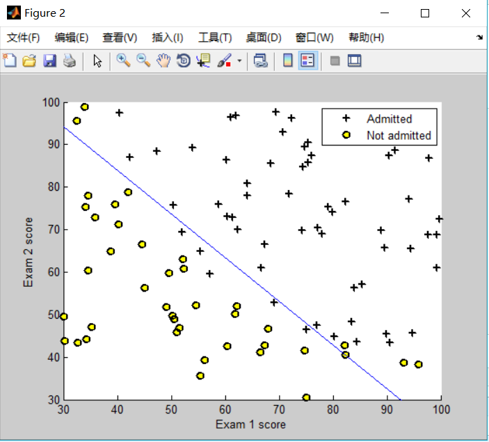
if size(X, 2) <= 3
    % Only need 2 points to define a line, so choose two endpoints 选择在坐标轴上的两个临界点
    plot_x = [min(X(:,2))-2,  max(X(:,2))+2];  

    % Calculate the decision boundary line theta(1) + theta(2) * x(1) + theta(3) * x(2) = 0 计算两个y在边界上的值
    plot_y = (-1./theta(3)).*(theta(2).*plot_x + theta(1));

    % Plot, and adjust axes for better viewing 两点确定一条直线
    plot(plot_x, plot_y)
    
    % Legend, specific for the exercise
    legend('Admitted', 'Not admitted', 'Decision Boundary')
    axis([30, 100, 30, 100])

predict. m 

 1 function p = predict(theta, X)
 2 %PREDICT Predict whether the label is 0 or 1 using learned logistic 
 3 %regression parameters theta
 4 %   p = PREDICT(theta, X) computes the predictions for X using a 
 5 %   threshold at 0.5 (i.e., if sigmoid(theta'*x) >= 0.5, predict 1)
 6 
 7 m = size(X, 1); % Number of training examples
 8 
 9 % You need to return the following variables correctly
10 p = zeros(m, 1);
11 
12 % ====================== YOUR CODE HERE ======================
13 % Instructions: Complete the following code to make predictions using
14 %               your learned logistic regression parameters. 
15 %               You should set p to a vector of 0's and 1's
16 %
17 
18 % cal h(x) -- predictions 
19 % pos = find(sigmoid( X * theta ) >= 0.5 );
20 % neg = find(sigmoid( x * theta ) < 0.5 );
21 p = sigmoid( X * theta ); 
22 for i = 1:m
23     if p(i) >= 0.5 
24         p(i) = 1;
25     else 
26         p(i) = 0;
27     end 
28 end 
29 % =========================================================================
30 end

 

ex2_reg. m 

  1 %% Machine Learning Online Class - Exercise 2: Logistic Regression
  2 %
  3 %  Instructions
  4 %  ------------
  5 %
  6 %  This file contains code that helps you get started on the second part
  7 %  of the exercise which covers regularization with logistic regression.
  8 %
  9 %  You will need to complete the following functions in this exericse:
 10 %
 11 %     sigmoid.m
 12 %     costFunction.m
 13 %     predict.m
 14 %     costFunctionReg.m
 15 %
 16 %  For this exercise, you will not need to change any code in this file,
 17 %  or any other files other than those mentioned above.
 18 %
 19 
 20 %% Initialization
 21 clear ; close all; clc
 22 
 23 %% Load Data
 24 %  The first two columns contains the X values and the third column
 25 %  contains the label (y).
 26 
 27 data = load('ex2data2.txt');
 28 X = data(:, [1, 2]); y = data(:, 3);
 29 
 30 plotData(X, y);
 31 
 32 % Put some labels
 33 hold on;
 34 
 35 % Labels and Legend
 36 xlabel('Microchip Test 1')
 37 ylabel('Microchip Test 2')
 38 
 39 % Specified in plot order
 40 legend('y = 1', 'y = 0')
 41 hold off;
 42 
 43 
 44 %% =========== Part 1: Regularized Logistic Regression ============
 45 %  In this part, you are given a dataset with data points that are not
 46 %  linearly separable. However, you would still like to use logistic
 47 %  regression to classify the data points.
 48 %
 49 %  To do so, you introduce more features to use -- in particular, you add
 50 %  polynomial features to our data matrix (similar to polynomial
 51 %  regression).
 52 %
 53 
 54 % Add Polynomial Features
 55 
 56 % Note that mapFeature also adds a column of ones for us, so the intercept
 57 % term is handled
 58 X = mapFeature(X(:,1), X(:,2));
 59 
 60 % Initialize fitting parameters
 61 initial_theta = zeros(size(X, 2), 1);
 62 
 63 % Set regularization parameter lambda to 1
 64 lambda = 1;
 65 
 66 % Compute and display initial cost and gradient for regularized logistic
 67 % regression
 68 [cost, grad] = costFunctionReg(initial_theta, X, y, lambda);
 69 
 70 fprintf('Cost at initial theta (zeros): %f\n', cost);
 71 fprintf('Expected cost (approx): 0.693\n');
 72 fprintf('Gradient at initial theta (zeros) - first five values only:\n');
 73 fprintf(' %f \n', grad(1:5));
 74 fprintf('Expected gradients (approx) - first five values only:\n');
 75 fprintf(' 0.0085\n 0.0188\n 0.0001\n 0.0503\n 0.0115\n');
 76 
 77 fprintf('\nProgram paused. Press enter to continue.\n');
 78 pause;
 79 
 80 % Compute and display cost and gradient
 81 % with all-ones theta and lambda = 10
 82 test_theta = ones(size(X,2),1);
 83 [cost, grad] = costFunctionReg(test_theta, X, y, 10);
 84 
 85 fprintf('\nCost at test theta (with lambda = 10): %f\n', cost);
 86 fprintf('Expected cost (approx): 3.16\n');
 87 fprintf('Gradient at test theta - first five values only:\n');
 88 fprintf(' %f \n', grad(1:5));
 89 fprintf('Expected gradients (approx) - first five values only:\n');
 90 fprintf(' 0.3460\n 0.1614\n 0.1948\n 0.2269\n 0.0922\n');
 91 
 92 fprintf('\nProgram paused. Press enter to continue.\n');
 93 pause;
 94 
 95 %% ============= Part 2: Regularization and Accuracies =============
 96 %  Optional Exercise:
 97 %  In this part, you will get to try different values of lambda and
 98 %  see how regularization affects the decision coundart
 99 %
100 %  Try the following values of lambda (0, 1, 10, 100).
101 %
102 %  How does the decision boundary change when you vary lambda? How does
103 %  the training set accuracy vary?
104 %
105 
106 % Initialize fitting parameters
107 initial_theta = zeros(size(X, 2), 1);
108 
109 % Set regularization parameter lambda to 1 (you should vary this)
110 lambda = 1;
111 
112 % Set Options
113 options = optimset('GradObj', 'on', 'MaxIter', 400);
114 
115 % Optimize
116 [theta, J, exit_flag] = ...
117     fminunc(@(t)(costFunctionReg(t, X, y, lambda)), initial_theta, options);
118 
119 % Plot Boundary
120 plotDecisionBoundary(theta, X, y);
121 hold on;
122 title(sprintf('lambda = %g', lambda))
123 
124 % Labels and Legend
125 xlabel('Microchip Test 1')
126 ylabel('Microchip Test 2')
127 
128 legend('y = 1', 'y = 0', 'Decision boundary')
129 hold off;
130 
131 % Compute accuracy on our training set
132 p = predict(theta, X);
133 
134 fprintf('Train Accuracy: %f\n', mean(double(p == y)) * 100);
135 fprintf('Expected accuracy (with lambda = 1): 83.1 (approx)\n');

costFunction_Reg.m 

 1 function [J, grad] = costFunctionReg(theta, X, y, lambda)
 2 %COSTFUNCTIONREG Compute cost and gradient for logistic regression with regularization
 3 %   J = COSTFUNCTIONREG(theta, X, y, lambda) computes the cost of using
 4 %   theta as the parameter for regularized logistic regression and the
 5 %   gradient of the cost w.r.t. to the parameters. 
 6 
 7 % Initialize some useful values
 8 m = length(y); % number of training examples
 9 
10 % You need to return the following variables correctly 
11 J = 0;
12 grad = zeros(size(theta));
13 
14 % ====================== YOUR CODE HERE ======================
15 % Instructions: Compute the cost of a particular choice of theta.
16 %               You should set J to the cost.
17 %               Compute the partial derivatives and set grad to the partial
18 %               derivatives of the cost w.r.t. each parameter in theta
19 alpha = 1;
20 other = lambda ./ (2 * m) * theta.^2 ; 
21 J = (-1/m) * ( y' * log(sigmoid(X * theta)) + ( 1-y )'* log(1-sigmoid(X*theta))) + other ;
22 grad = ( alpha / m ) * X'* (sigmoid( X * theta ) - y) + lambda ./ m * theta ;
23 
24 % =============================================================
25 
26 end

 

转载于:https://www.cnblogs.com/twomeng/p/9533429.html