matlab教程中包含emd,Empirical mode decomposition

Simulate a vibration signal from a damaged bearing. Perform empirical mode decomposition to visualize the IMFs of the signal and look for defects.

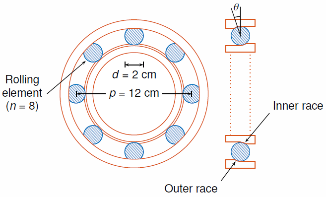
A bearing with a pitch diameter of 12 cm has eight rolling elements. Each rolling element has a diameter of 2 cm. The outer race remains stationary as the inner race is driven at 25 cycles per second. An accelerometer samples the bearing vibrations at 10 kHz.

fs = 10000;

f0 = 25;

n = 8;

d = 0.02;

p = 0.12;

The vibration signal from the healthy bearing includes several orders of the driving frequency.

t = 0:1/fs:10-1/fs;

yHealthy = [1 0.5 0.2 0.1 0.05]*sin(2*pi*f0*[1 2 3 4 5]'.*t)/5;

A resonance is excited in the bearing vibration halfway through the measurement process.

yHealthy = (1+1./(1+linspace(-10,10,length(yHealthy)).^4)).*yHealthy;

The resonance introduces a defect in the outer race of the bearing that results in progressive wear. The defect causes a series of impacts that recur at the ball pass frequency outer race (BPFO) of the bearing:

BPFO=12nf0[1-dpcosθ],

where f0 is the driving rate, n is the number of rolling elements, d is the diameter of the rolling elements, p is the pitch diameter of the bearing, and θ is the bearing contact angle. Assume a contact angle of 15° and compute the BPFO.

ca = 15;

bpfo = n*f0/2*(1-d/p*cosd(ca));

Use the pulstran function to model the impacts as a periodic train of 5-millisecond sinusoids. Each 3 kHz sinusoid is windowed by a flat top window. Use a power law to introduce progressive wear in the bearing vibration signal.

fImpact = 3000;

tImpact = 0:1/fs:5e-3-1/fs;

wImpact = flattopwin(length(tImpact))'/10;

xImpact = sin(2*pi*fImpact*tImpact).*wImpact;

tx = 0:1/bpfo:t(end);

tx = [tx; 1.3.^tx-2];

nWear = 49000;

nSamples = 100000;

yImpact = pulstran(t,tx',xImpact,fs)/5;

yImpact = [zeros(1,nWear) yImpact(1,(nWear+1):nSamples)];

Generate the BPFO vibration signal by adding the impacts to the healthy signal. Plot the signal and select a 0.3-second interval starting at 5.0 seconds.

yBPFO = yImpact + yHealthy;

xLimLeft = 5.0;

xLimRight = 5.3;

yMin = -0.6;

yMax = 0.6;

plot(t,yBPFO)

hold on

[limLeft,limRight] = meshgrid([xLimLeft xLimRight],[yMin yMax]);

plot(limLeft,limRight,'--')

hold off

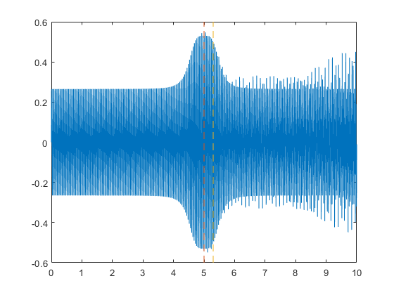
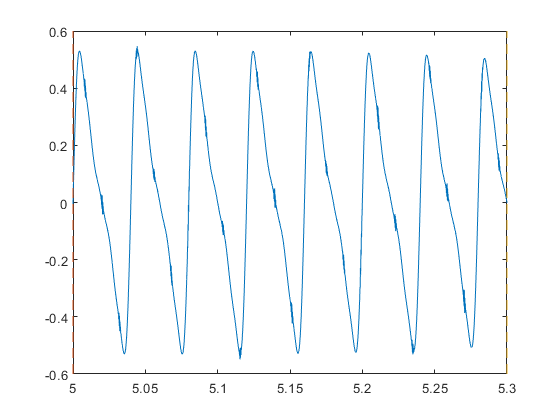
Zoom in on the selected interval to visualize the effect of the impacts.

xlim([xLimLeft xLimRight])

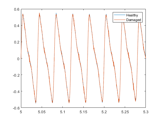
Add white Gaussian noise to the signals. Specify a noise variance of 1/1502.

rn = 150;

yGood = yHealthy + randn(size(yHealthy))/rn;

yBad = yBPFO + randn(size(yHealthy))/rn;

plot(t,yGood,t,yBad)

xlim([xLimLeft xLimRight])

legend('Healthy','Damaged')

Use emd to perform an empirical mode decomposition of the healthy bearing signal. Compute the first five intrinsic mode functions (IMFs). Use the 'Display' name-value pair to show a table with the number of sifting iterations, the relative tolerance, and the sifting stop criterion for each IMF.

imfGood = emd(yGood,'MaxNumIMF',5,'Display',1);

Current IMF | #Sift Iter | Relative Tol | Stop Criterion Hit

1 | 3 | 0.017132 | SiftMaxRelativeTolerance

2 | 3 | 0.12694 | SiftMaxRelativeTolerance

3 | 6 | 0.14582 | SiftMaxRelativeTolerance

4 | 1 | 0.011082 | SiftMaxRelativeTolerance

5 | 2 | 0.03463 | SiftMaxRelativeTolerance

Decomposition stopped because maximum number of intrinsic mode functions was extracted.

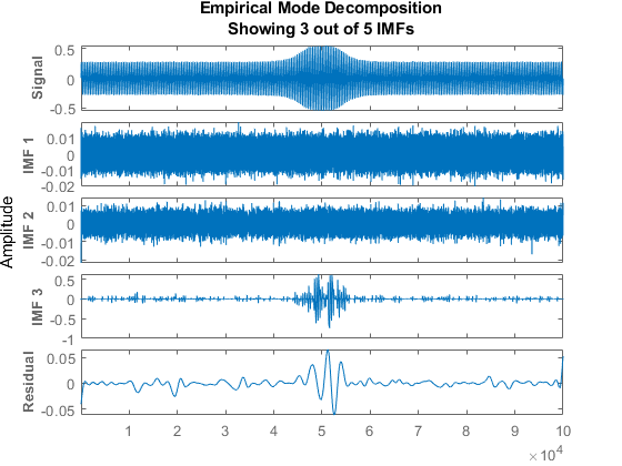
Use emd without output arguments to visualize the first three modes and the residual.

emd(yGood,'MaxNumIMF',5)

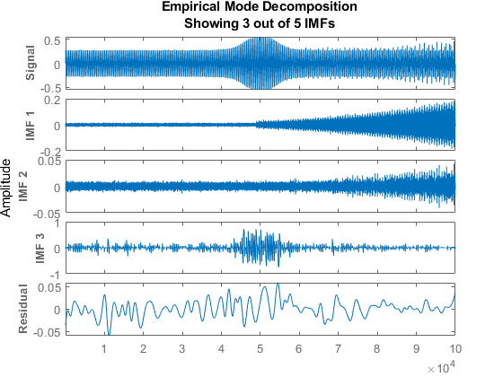
Compute and visualize the IMFs of the defective bearing signal. The first empirical mode reveals the high-frequency impacts. This high-frequency mode increases in energy as the wear progresses. The third mode shows the resonance in the vibration signal.

imfBad = emd(yBad,'MaxNumIMF',5,'Display',1);

Current IMF | #Sift Iter | Relative Tol | Stop Criterion Hit

1 | 2 | 0.041274 | SiftMaxRelativeTolerance

2 | 3 | 0.16695 | SiftMaxRelativeTolerance

3 | 3 | 0.18428 | SiftMaxRelativeTolerance

4 | 1 | 0.037177 | SiftMaxRelativeTolerance

5 | 2 | 0.095861 | SiftMaxRelativeTolerance

Decomposition stopped because maximum number of intrinsic mode functions was extracted.

emd(yBad,'MaxNumIMF',5)

The next step in the analysis is to compute the Hilbert spectrum of the extracted IMFs. For more details, see the Compute Hilbert Spectrum of Vibration Signal example.