线性拟合polyfit_Python曲线拟合详解

最新推荐文章于 2024-04-25 23:56:51 发布

橙小知

最新推荐文章于 2024-04-25 23:56:51 发布

阅读量1.1w

点赞数 6

文章标签：线性拟合polyfit

本文链接：https://blog.csdn.net/weixin_34746495/article/details/112668110

版权

转一个超级详细的Python曲线拟合详解文章（怕以后找不到了），本栏目初学者不用细看，当手册查就好了。原文在这里：04.04 curve fitting，侵删。

导入基础包：

In [1]:

import numpy as np
import matplotlib as mpl
import matplotlib.pyplot as plt

导入线多项式拟合工具：

In [2]:

from numpy import polyfit, poly1d

产生数据：

In [3]:

x = np.linspace(-5, 5, 100)
y = 4 * x + 1.5
noise_y = y + np.random.randn(y.shape[-1]) * 2.5

画出数据：

In [4]:

%matplotlib inline

p = plt.plot(x, noise_y, 'rx')
p = plt.plot(x, y, 'b:')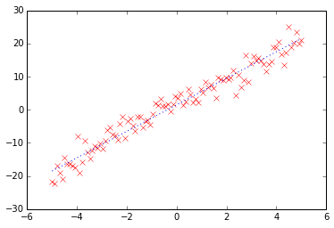

进行线性拟合，polyfit 是多项式拟合函数，线性拟合即一阶多项式：

In [5]:

coeff = polyfit(x, noise_y, 1)
print coeff

[ 3.93921315  1.59379469]

一阶多项式 y=a1x+a0 拟合，返回两个系数 [a1,a0]。

画出拟合曲线：

In [6]:

p = plt.plot(x, noise_y, 'rx')
p = plt.plot(x, coeff[0] * x + coeff[1], 'k-')
p = plt.plot(x, y, 'b--')

还可以用 poly1d 生成一个以传入的 coeff 为参数的多项式函数：

In [7]:

f = poly1d(coeff)
p = plt.plot(x, noise_y, 'rx')
p = plt.plot(x, f(x))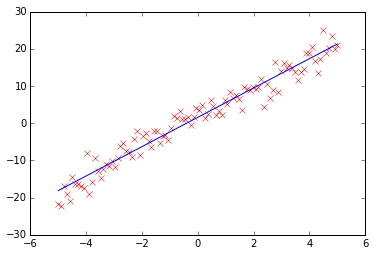

In [8]:

关注