


INTRODUCTION 引言
The numerical techniques introduced in this chapter involve the use of Laplace transforms for manipulating and displaying differential equations and numerical integration for solving the differential equations. These techniques form the basis of all of the numerical methods used throughout the text. A numerical example will be presented that will illustrate a practical application of the use of Laplace transforms and numerical integration. Another example will be presented showing how z transforms can be used to both represent difference equations and get their solution.
本章介绍的数值运算技术包括,使用拉普拉斯变换方法来实现对微分方程的表示和操作,以及使用数值积分方法来求解微分方程。这些数值运算技术构成了本文涉及到所有数值方法的基础。本章首先将给出一个数值运算示例,说明拉普拉斯变换和数值积分的实际应用;随后将给出另一个示例,说明如何使用z变换方法来表示差分方程并求得方程的解。
LAPLACE TRANSFORMS AND DIFFERENTIAL EQUATIONS 拉普拉斯变换与微分方程
Transform methods are often useful because certain operations in one domain are different and often simpler than operations in the other domain. For example, ordinary differential equations in the time domain become algebraic expressions in the s domain after being Laplace transformed. In control system engineering, Laplace transforms are used both as a shorthand notation and as a method for solving linear differential equations. In this text we will frequently use Laplace transform notation to represent subsystem dynamics in tactical missile guidance systems.
If we define F(s) as the Laplace transform of f(t), then the Laplace transform has the following definition
拉普拉斯变换方法具有很高的实用性。对于某个确定的运算在不同域中的操作是不同的,而且通常情况下选择在某个域中完成这个运算会更加简便。例如,时域中的常微分方程经过拉普拉斯变换后,变为了s域中的代数方程。在控制系统工程中,拉普拉斯变换既被用作速记符号,也被用作求解线性微分方程的方法。在本书中,我们将频繁使用拉普拉斯变换表示法来描述战术导弹制导系统中各子系统的动力学。
如果我们将F(s)定义为f(t)的拉普拉斯变换,则拉普拉斯变换具有以下定义
F ( s ) = ∫ 0 ∞ f ( t ) e − s t d t F(s) = \int_{0}^{\infin} f(t) e^{-st}dt F(s)=∫0∞f(t)e−stdt
With this definition it is easy to show that a summation in the time domain is also a summation in the Laplace transform or frequency domain. For example, if
f
1
(
t
)
f _1 (t)
f1(t)and
f
2
(
t
)
f_2 (t)
f2(t)have Laplace transforms
F
1
(
s
)
F_1 (s)
F1(s)and
F
2
(
s
)
F_2 (s)
F2(s), respectively, then
根据上述定义可以很轻易的得知,时域中多项之和的拉普拉斯变换等于时域中各项拉普拉斯变化结果之和。比如,如果
f
1
(
t
)
f _1 (t)
f1(t)和$f_2 (t)的拉普拉斯变化分别为
F
1
(
s
)
F_1(s)
F1(s) 和
F
2
(
s
)
F_2 (s)
F2(s),则:
L [ f 1 ( t ) ± f 2 ( t ) ] = F 1 ( s ) ± F 2 ( s ) \mathscr{L}[f_1(t) \pm f_2(t)] = F_1(s) \pm F_2(s) L[f1(t)±f2(t)]=F1(s)±F2(s)
译者注:拉普拉斯变换,简称为“拉式变换”
译者注:和 的 拉氏变换 = 拉氏变换 的 和。
Again, using the definition of the Laplace transform, it is easy to show that differentiation in the time domain is equivalent to frequency multiplication in the Laplace transform domain, or
继续根据拉普拉斯变换的定义可以的得知,时域中的求导运算,等价于拉普拉斯域中的乘法运算。或:
L ( d f ( t ) d t ) = s F ( s ) − f ( 0 ) \mathscr{L}(\frac{df(t)}{dt}) = sF(s) - f(0) L(dtdf(t))=sF(s)−f(0)
where f(0) is the initial condition on f(t). The Laplace transform of the
n
t
h
n^{th}
nth derivative of a function is given by
其中 f(0) 是 f(t) 的初始值。 函数的n阶导数的拉普拉斯变换由下式给出:
L ( d n f ( t ) d t n ) = s n F ( s ) − s n − 1 f ( 0 ) − s n − 2 d f ( 0 ) d t − . . . \mathscr{L}(\frac{d^{n}f(t)}{dt^{n}}) = s^{n}F(s) -s^{n-1} f(0)-s^{n-2} \frac{df(0)}{dt} - ... L(dtndnf(t))=snF(s)−sn−1f(0)−sn−2dtdf(0)−...
From the preceding equation we can see that, for zero initial conditions, the n^{th} derivative in the time domain is equivalent to a multiplication by s n in the Laplace transform domain.
从上述公式可以看出,对于零初始状态,时域中的n阶求导运算,等价于拉普拉斯域中与s的n此乘法运算。
译者注:将问题从时域转到频域中可以用代数的方式解决微积分的问题,极大的简化了运算难度。
译者注:拉普拉斯变换域,也称为“复数域”或者“s域”,为了方便描述,且与国内教材保持一致,后统称为“复数域”
Laplace transforms can also be used to convert the input-output relationship of a differential equation to a shorthand notation called a transfer function representation. For example, given the second-order equation
拉普拉斯变换也可用做将微分方程的输入-输出关系转化为一种叫做传递函数 的速记符号,比如对于二阶微分方程。
d 2 y ( t ) d t 2 + 2 d y ( t ) d t + 4 y ( t ) = x ( t ) \frac{d^2y(t)}{dt^2} + 2\frac{dy(t)}{dt} + 4y(t) = x(t) dt2d2y(t)+2dtdy(t)+4y(t)=x(t)
with zero initial conditions, or
满足零初始状态条件,或
d y ( 0 ) d t = 0 , y ( 0 ) = 0 \frac{dy(0)}{dt} = 0 \quad,\quad y(0) = 0 dtdy(0)=0,y(0)=0
we can find the same differential equation in the Laplace transform domain to be
我们可以在复数域中找到该微分方程的等价表达式。
s 2 Y ( s ) + 2 s Y ( s ) + 4 Y ( s ) = X ( s ) s^2Y(s) + 2sY(s) + 4Y(s) = X(s) s2Y(s)+2sY(s)+4Y(s)=X(s)
Combining like terms in the preceding equation to get a fractional relationship between the output and input, known as a transfer function, yields
对上式进行同类项合并,可得到一个分数形式的输入-输出关系式,被称作传递函数,即
Y ( s ) X ( s ) = 1 s 2 + 2 s + 4 \frac{Y(s)}{X(s)} = \frac{1}{s^2 +2s +4} X(s)Y(s)=s2+2s+41
Similarly, given a transfer function, we can go back to the differential equation form. Consider the second-order transfer function
类似,在给定传递函数的情况下,可以反向转化为微分方程的形式。考虑二阶传递函数。
Y ( s ) X ( s ) = 1 + 2 s 1 + 2 s + s 2 \frac{Y(s)}{X(s)} = \frac{1 + 2s}{1 + 2s + s^2} X(s)Y(s)=1+2s+s21+2s
We know that , according to the chain rule , the transfer function can be expressed as
众所周知,根据链式法则,传递函数可以被表示为
Y ( s ) X ( s ) = E ( s ) X ( s ) Y ( s ) E ( s ) \frac{Y(s)}{X(s)} = \frac{E(s)}{X(s)}\frac{Y(s)}{E(s)} X(s)Y(s)=X(s)E(s)E(s)Y(s)
Therefore, we can break the relationship into the following two equivalent transfer functions:
因此,可以将上述关系式拆解成如下两个等价的的传递函数
E ( s ) X ( s ) = 1 1 + 2 s + s 2 , Y ( s ) E ( s ) = 1 + 2 s \frac{E(s)}{X(s)}= \frac{1}{1 + 2s + s^2}\quad,\quad\frac{Y(s)}{E(s)}= 1+ 2s X(s)E(s)=1+2s+s21,E(s)Y(s)=1+2s
Cross multiplication results in
交叉相乘后得到
s 2 E ( s ) + 2 s E ( s ) + E ( s ) = X ( s ) s^2E(s) + 2sE(s) + E(s) = X(s) s2E(s)+2sE(s)+E(s)=X(s)
and
和
2 s E ( s ) + E ( s ) = Y ( s ) 2sE(s) + E(s) =Y(s) 2sE(s)+E(s)=Y(s)
Converting the first equation to the time domain yields the second-order differential equation
将第一个方程转换到时域中得到如下二阶微分方程
d 2 e ( t ) d t 2 + 2 d e ( t ) d t + e ( t ) = x ( t ) \frac{d^2e(t)}{dt^2} + 2\frac{de(t)}{dt}+e(t) = x(t) dt2d2e(t)+2dtde(t)+e(t)=x(t)
and converting the second equation yields the output relationship
转化第二个方程得到如下输出关系
y ( t ) = 2 d e ( t ) d t + e ( t ) y(t) = 2\frac{de(t)}{dt} + e(t) y(t)=2dtde(t)+e(t)
The implication from the transfer function notation is that the initial conditions on the second-order differential equation are zero, or
传递函数表示的一个隐含条件是二阶微分方程的初始条件为零,或
d e ( 0 ) d t = 0 , e ( 0 ) = 0 \frac{de(0)}{dt} = 0\quad,\quad e(0)=0 dtde(0)=0,e(0)=0
Often we will use Laplace transform notation and, for shorthand, drop the functional dependence on s in the notation [that is, F is equivalent to F(s)]. Similarly, when we are in the time domain, the functional dependence on t will often be dropped [that is, f is equivalent to f(t)]. In addition, block diagrams and program listings will frequently use the overdot notation to represent time derivatives. With this notation, each overdot represents a derivative. For example,
使用拉式变换表示法会被频繁使用,为了简化,去掉拉普拉斯表示法中的字母s[即,F等价于F(s)]。类似地,在时域表达式中通常会省略字母t[即,f 等价于f(t)]。此外,在框图和程序列表中将经常使用字母点上标来表示对时间的导数,每一个点表示一次对时间的求导。例如
y ˙ = d y d t , y ¨ = d 2 y d t 2 , y ˉ = d 3 y d t 3 \dot{y} = \frac{dy}{dt},\quad \ddot{y} = \frac{d^2y}{dt^2},\quad \bar{y} = \frac{d^3y}{dt^3} y˙=dtdy,y¨=dt2d2y,yˉ=dt3d3y
Therefore, converting to the overdot notation yields
因此,将下式转化为使用点上标表示的表示方式
d 2 e ( t ) d t 2 + 2 d e ( t ) d t + e ( t ) = x ( t ) \frac{d^2e(t)}{dt^2} + 2\frac{de(t)}{dt}+e(t) = x(t) dt2d2e(t)+2dtde(t)+e(t)=x(t)
e ¨ + 2 e ˙ + e = x \ddot{e}+2\dot{e}+e = x e¨+2e˙+e=x
Occasionally, we shall either convert time functions to Laplace transforms or vice versa, by inspection. Some common transfer functions [1], along with their time domain equivalents, appear in Table 1.1. A more extensive listing of inverse Laplace transforms can be found in [1].
偶尔可以通过查表法实现时域到复数域的转化(或者从复数域到时域的转化)。表1.1中列出了一些常见的传递函数[1]及其时域等效函数。在参考文献[1]中可以找到更全面的拉式逆变换列表。
表1.1 常用拉式反变换表
| F ( s ) F(s) F(s) | f(t) |
|---|---|
| K s \frac{K}{s} sK | K |
| K s n \frac{K}{s^n} snK | K t n − 1 ( n − 1 ) ! \frac{Kt^{n-1}}{(n-1)!} (n−1)!Ktn−1 |
| K ( s − a ) n \frac{K}{(s-a)^n} (s−a)nK | K t n − 1 e a t ( n − 1 ) ! \frac{Kt^{n-1}e^{at}}{(n-1)!} (n−1)!Ktn−1eat |
| K s 2 + a 2 \frac{K}{s^2+a^2} s2+a2K | K s i n ( a t ) a \frac{Ksin(at)}{a} aKsin(at) |
| K s s 2 + a 2 \frac{Ks}{s^2+a^2} s2+a2Ks | K c o s ( a t ) Kcos(at) Kcos(at) |
| K ( s − a ) 2 + b 2 \frac{K}{(s-a)^2+b^2} (s−a)2+b2K | K e a t s i n ( b t ) b \frac{Ke^{at}sin(bt)}{b} bKeatsin(bt) |
| K ( s − a ) ( s − a ) 2 + b 2 \frac{K(s-a)}{(s-a)^2+b^2} (s−a)2+b2K(s−a) | K a a t c o s ( b t ) Ka^{at}cos(bt) Kaatcos(bt) |
NUMERICAL INTEGRATION OF DIFFERENTIAL EQUATIONS 微分方程的数值积分
Throughout this text we will be simulating both linear and nonlinear ordinary differential equations. Because, in general, these equations have no closed-form solutions, it will be necessary to resort to numerical integration techniques to solve or simulate these equations. Many numerical integration techniques [2] exist for solving differential equations. However, we shall use the second-order Runge–Kutta technique throughout the text because it is simple to understand, easy to program, and, most importantly, yields accurate answers for all of the examples presented in this text.
在本文中,我们将对线性和非线性常微分方程进行仿真模拟。通常这些方程没有闭式解,因此采用数值积分技术来对这些方程进行仿真和求解是很有必要的。很多的数值积分技术[2]都可用于求解微分方程,为了方便理解和编程实现,且保证解的准确性,本文的所有实例都将使用二阶Runge–Kutta法作为求解方法。
译者注:数值积分的思路是使用迭代的方式求取微分方程的解,这部分知识属于《数值分析》领域,是研究生必修课程。
译者注:Runge–Kutta法 通常翻译为“龙格库塔法”是一种高精度的数值积分方法。常见的数值积分方法还有欧拉法、拉格朗日法等。
The second-order Runge–Kutta numerical integration procedure is easy to state. Given a first-order differential equation of the form
二阶Runge–Kutta法的数值积分步骤简单易述。对于给出的一阶微分方程
x ˙ = f ( x , t ) \dot{x} = f(x,t) x˙=f(x,t)
where t is time, we seek to find a recursive relationship for x as a function of time. With the second-order Runge–Kutta numerical technique, the value of x at the next integration interval h is given by
其中t表示时间,下面需要求取关于时间t函数x的递归关系。利用二阶Runge–Kutta数值积分方法,x在下一个积分间隔h中的值为
x K + 1 = x K + h f ( x , t ) 2 + h f ( x , t + h ) 2 x_{K+1} = x_K +\frac{hf(x,t)}{2}+\frac{hf(x,t+h)}{2} xK+1=xK+2hf(x,t)+2hf(x,t+h)
where the subscript K represents the last interval and K + 1 represents the new interval. From the preceding expression we can see that the new value of x is simply the old value of x plus a term proportional to the derivative evaluated at time t and another term with the derivative evaluated at time t + h.
其中,K表示上一个积分间隔,K+1表示心得积分间隔。从上述表达式中可以看出,x的新值就是在x的旧值基础上单的叠加两个与x导数成比例的项,其中一项是在t时刻对x导数的估计值,另外一项是在t+h时刻对x导数的估计值。
The integration step size h must be small enough to yield answers of sufficient accuracy. A simple test, commonly practiced among engineers, is to find the appropriate integration step size by experiment. As a rule of thumb, the initial step size is chosen to be several times smaller than the smallest time constant in the system under consideration. The step size is then halved to see if the answers change significantly. If the new answers are approximately the same, the larger integration step size is used to avoid excessive computer running time. If the answers change substantially, then the integration interval is again halved and the process is repeated.
为了得到足够精确的仿真结果,积分步长h必须选择一个足够小的值。工程师们通常会进行的一个简单测试,以仿真实验的方式确定合适的积分步长。作为经验,初始步长可选为所研究系统中最小时间常数的n分之一,然后将步长减半,以查看步长减半前后的仿真结果是否有显著变化。如果新旧结果大致相同,则选用两者中更大的积分步长,以避免过长的计算机运行时间。如果新旧结果有显著的不同,则需将积分步长再次减半,并重复上述过程。
To see how the Runge–Kutta technique can be applied to a practical example, let us consider the problem of finding the step response of one of the second-order networks from Table 1.1. Consider the sinusoidal transfer function
为了更好的说明Runge–Kutta法在实际问题中的应用,以"求取一个二阶系统的阶跃响应"问题为例。从表1.1中选取正弦函数的传递函数作为研究对象
Y X = ω s 2 + ω 2 \frac{Y}{X} = \frac{\omega}{s^2+\omega^2} XY=s2+ω2ω
where X is the input, Y the output, ω \omega ω the natural frequency of the second-order network, and s the Laplace transformation notation for a derivative. Cross multiplying the numerator and denominator of the transfer function and solving for the highest derivative, as was shown in the previous section, yields the following second-order differential equation:
其中X是输入,Y是输出, ω \omega ω是二阶系统的自然频率,s是求导运算的拉氏变换符。如上一节所示,将传递函数的分子和分母交叉相乘并求解出最高次导数,得到以下二阶微分方程:
y ¨ = ω x − ω 2 y \ddot{y} = \omega x -\omega^2y y¨=ωx−ω2y
where the double overdot represents two differentiations.
其中,上标两个点表示求两次微分。
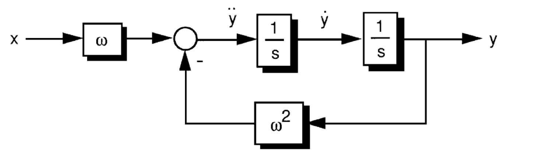 Fig. 1.1 Block diagram representation of second-order system. 图.1.1 二阶系统框图
This second-order differential equation can be represented in block diagram form as shown in Fig. 1.1. In this diagram each 1/s represents an integration. The outputs of each integrator are sometimes called states and are y and y dot respectively.
该二阶微分方程可用如图1.1所示的框图表示。图中,每个1/s代表一次积分。每个积分器的输出值有时被称为状态量,该系统的状态量分别为
y
y
y和
y
˙
\dot{y}
y˙。
If x is a step input in Fig. 1.1, we can find the response y exactly using Laplace transform techniques. Recall from Table 1.1 that 1/s represents a step function in the Laplace transform domain. Therefore we can express the output y in the Laplace transform domain as
如果图1.1中的输入信号x为阶跃信号,则可以使用拉式变换法得到输出信号y的精确解。回顾表1.1可知1/s在复数域中表示阶跃信号。因此,可以将复数域中的输出y表示为
Y ( s ) = ω s ( s 2 + ω 2 ) Y(s) = \frac{\omega}{s(s^2+\omega^2)} Y(s)=s(s2+ω2)ω
Expanding the preceding expression using partial fraction expansion yields
使用部分分数展开法展开上述表达式后得到
Y ( s ) = 1 ω [ 1 s − s s 2 + ω 2 ] Y(s) = \frac{1}{\omega}[\frac{1}{s} - \frac{s}{s^2 + \omega^2}] Y(s)=ω1[s1−s2+ω2s]
The inverse Laplace transform of Y(s) produces y in the time domain or y(t). The output can be found by using Table 1.1 obtaining
对Y(s)进行拉式逆变换得到时域中的y或y(t)。可通过查询表1.1可得输出信号为
y = 1 ω ( 1 − c o s ω t ) y = \frac{1}{\omega}(1- cos\omega t) y=ω1(1−cosωt)
To check the preceding theoretical closed-form solution for y, a simulation involving numerical integration was written based on the system of Fig. 1.1. A simulation of the second-order system, using the second-order Runge–Kutta integration techniques, appears in Listing 1.1. We can see from the listing that the second-order differential equation, or derivative information, appears just before the FLAG=1 statement. We come to this code twice during the integration interval: once to evaluate the derivative at time t and once to evaluate the derivative at time t + h. We can also see from Listing 1.1 that every 0.01 s we print out the output along with the closed-form solution. In this particular example the natural frequency ω \omega ω of the second-order system is 20 rad/s.
为了检验上文推导y的闭式理论解,本节基于图1.1所述系统编写了一个数值积分的仿真程序。使用二阶Runge–Kutta积分法对二阶系统进行求解仿真的代码如表1.1所示。语句FLAG = 1的前一句代码表示二阶微分方程(导数信息)。
一次在计算t时刻的导数,另一次在计算t+h时刻的导数。我们还可以从表1.1中看到,每0.01秒,程序会将数值积分的输出与推导出的封式理论解一起打印出来。在本示例中,二阶系统的固有频率
ω
\omega
ω 为20rad/s。
We can see from Listing 1.1 that the integration step size h is 0.001 s. Because the simulation time is 1 s, the ratio of the simulation time to the step size is 1000. This means that 2000 passes are made to the differential equations. The resultant system transient response, due to a step input (x ¼1), is shown in Fig. 1.2. We can see that the simulation output agrees exactly with the closed-form solution.
close all
clc
T=0.;% 仿真时钟
S=0.;% 存数时钟
Y=0.;% 状态量1
YD=0.;% 状态量2
X=1.;
H=.001;% 数值积分步长
n=0.;
W=20;				% 译者增加,系统参数:自由震荡频率 rad/s
while T <=(1.-1e-5)
    YOLD=Y;             % 记录当前状态量1
    YDOLD=YD;           % 记录当前状态量2
    STEP=1;             % 局部运算次数标志
    FLAG=0;             % 已经更新状态微分标志
    while STEP <=1      %
        if FLAG==1      % 已经更新状态微分
            STEP=2;     %
            Y=Y+H*YD;   % 利用微分更新状态量1
            YD=YD+H*YDD;% 利用微分更新状态量2
            T=T+H;      % 更新时间
        end
        YDD=W*X-W*W*Y;	%微分方程:由状态量求状态微分
        FLAG=1;
    end
    FLAG=0;
    Y=.5*(YOLD+Y+H*YD);	   % 二阶Runge–Kutta积分:旧值+0.5t时刻估计+0.5t+h时刻估计
    YD=.5*(YDOLD+YD+H*YDD);% 二阶Runge–Kutta积分:旧值+0.5t时刻估计+0.5t+h时刻估计
    S=S+H;% 数据存数周期控制
    if S >=.000999 % 数据存数流程
        S=0.;
        n=n+1;
        ArrayT(n)=T;% 记录当前时刻
        ArrayY(n)=Y;% 记录数值积分输出值
    end
end
figure

plot(ArrayT,ArrayY),grid  % 绘制数值积分结果
xlabel('Time (Sec)')
ylabel('y')

%% 译者加入:绘制拉氏变换推导的理论闭式解
ArrayY_ = 1/W*(1-cos(W*ArrayT));
hold on
plot(ArrayT,ArrayY_,'--','LineWidth',2)
legend('Runge–Kutta','Closed-Form solution')
%%

clc
output=[ArrayT',ArrayY',ArrayY_'];   % 译者更改:同时保存闭式解和数值解
save datfil.txt output  -ascii
disp 'simulation finished'
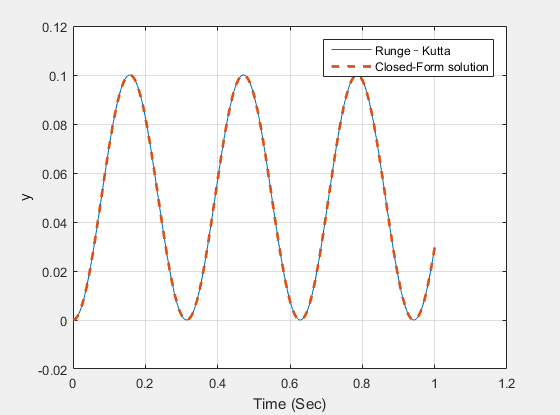
Fig. 1.2 Numerically integrating differential equations yields same results as closed-form solution.
图.1.2 微分方程数值积分的解与闭式解
译者注:上文说明了数值积分方法的合理性和准确性。从图中可以看出,采用二阶Runge–Kutta数值积分法得到的微分方程的解与理论推导所得解高度吻合,因此二阶Runge–Kutta数值积分方法可以用于微分方程组的求解。
Z TRANSFORMS AND DIFFERENCE EQUATIONS z-变换和差分方程
We have already shown that Laplace transforms are a useful way of representing differential equations. In this text we shall also want to simulate difference equations. Z transforms can also be used as an engineering shorthand for representing the difference equations. Later in this section we will also show how Z transforms can be used to solve difference equations and sometimes check simulation results [3].
我们已经说明拉氏变换是一种表示微分微分方程的常用方法。同样,在这一bufen 我们也想对差分方程进行仿真。Z变换同样也可被当做一种表示差分方程的工程技巧。在本节中我们会说明Z变换是如何被用于求解差分方程的,并且会通过仿真验证求解结果的正确性。
If we define F(z) as the Z transform of f (n), then the Z transform has the following definition:
如果定义F(z)为f(n)的Z变换,则Z变换定义如下:
F ( z ) = ∑ n = 0 ∞ f ( n ) z − n F(z) = \sum_{n= 0}^{ \infin}f(n)z^{-n} F(z)=n=0∑∞f(n)z−n
With this definition it is easy to show that a summation in the time or n domain is also a summation in the Z transform domain. For example, if
f
1
(
n
)
f_1 (n)
f1(n) and
f
2
(
n
)
f_2 (n)
f2(n) have Z transforms
F
1
(
z
)
F_1 (z)
F1(z)and
F
2
(
z
)
F_2 (z)
F2(z), respectively, then
根据这个定义,很容易得知,时域(n域)的和对应Z变换域中的和。比如,如果
f
1
(
n
)
f_1 (n)
f1(n) 和
f
2
(
n
)
f_2 (n)
f2(n) 的Z变换分别为
F
1
(
z
)
F_1 (z)
F1(z)和
F
2
(
z
)
F_2 (z)
F2(z),则
Z [ f 1 ( n ) ± f 2 ( n ) ] = F 1 ( z ) ± F 2 ( z ) Z[f_1(n) \pm f_2(n)] = F_1(z) \pm F_2(z) Z[f1(n)±f2(n)]=F1(z)±F2(z)
译者注:
和的Z变换=Z变换的和
One can show that the Z transform of a signal at time n + 1 is a multiplication of the function in the Z transform domain by z. The Z transform of the signal at time n according to
有一件事是可以明确的,信号在n+1时刻的Z变换等于信号在n时刻的Z变换结果乘以z,信号在n+1时刻的Z变换结果为
Z ( f n + 1 ) = z F ( z ) − z f ( 0 ) Z(f_{n+1} )= zF(z) - zf(0) Z(fn+1)=zF(z)−zf(0)
where f(0) is an initial condition. Often we will be working with systems having zero initial conditions.
其中f(0)为初始状态。通常情况下我们研究的系统都是0初始状态。
A list of some common Z transforms can be found in Table 1.2. From the table we can see that there is a relationship between the sampling time
T
s
T_s
Ts and time t given by
表1.2中列举了若干常见的Z变换公式。从表中可以看出,采样周期
T
s
T_s
Ts 和时间
t
t
t 之间存在如下关系
t = n T s t= nT_s t=nTs
TABLE 1.2 Z TRANSFORMS OF COMMON FUNCTIONS
表1.2 常见方程的Z变换表
| Function | Z transform |
|---|---|
| δ ( n ) \delta(n) δ(n) | 1 |
| 1 1 1 | z / ( z − 1 ) z/(z-1) z/(z−1) |
| a n a^n an | z / ( z − a ) z/(z-a) z/(z−a) |
| n n n | z / ( z − 1 ) 2 z/(z-1)^2 z/(z−1)2 |
| s i n ω n T s sin \omega nT_s sinωnTs | z s i n ω T s / ( z 2 − 2 z c o s ω T s + 1 ) z sin\omega T_s/(z^2-2zcos\omega T_s +1) zsinωTs/(z2−2zcosωTs+1) |
To illustrate how Z transforms can be used to solve difference equations, let us consider a numerical example involving the fading memory filters we will be working with in Chapter 7. The simplest fading memory filter can be expressed as the difference equation
为了说明Z变换是如何被用于差分方程求解的,我们以本书第七章会涉及到的渐消记忆滤波器作为一个数值积分的案例。最简单的渐消记忆滤波器可以被表示为如下的差分方程。
y n + 1 = y n + G ( x n + 1 − y n ) y_{n+1} = y_n +G(x_{n+1} - y_n) yn+1=yn+G(xn+1−yn)
where y is the filter estimate or output, x is the filter input or measurement, and G the filter gain. For the first-order fading memory filter, the filter gain is a designer chosen number between zero and unity. We can find the filter response to a step input (that is, x n + 1 = 1 x_{n+1} =1 xn+1=1) by observing from Table 1.2 that the Z transform of a unit step function or constant is given by
其中y是滤波器估计值(或输出值),x是滤波器输量(或测量值),G是滤波器增益。对于一阶衰减记忆滤波器,滤波器增益是设计者所选的一个介于0和1之间的数字。通过参考表1.2中单位阶跃函数(或常值)的Z变换,我们可以得到滤波器对阶跃信号(即
x
n
+
1
=
1
x_{n+1} =1
xn+1=1)的响应。
z ( 1 ) = z / ( z − 1 ) z(1) = z/(z-1) z(1)=z/(z−1)
Therefore taking the Z transform of both sides of the difference equation yields
因此对差分方程两边同时进行Z变换,得到:
z Y = Y + G ( z z − 1 − Y ) zY = Y +G(\frac{z}{z-1}-Y) zY=Y+G(z−1z−Y)
If we bring all the terms in Y to the left-hand side of the equation, we get
如果我们将所有与Y相关的项都移到等式左侧,得到:
Y ( z − 1 + G ) = G z / ( z − 1 ) Y(z-1+G) = Gz/(z-1) Y(z−1+G)=Gz/(z−1)
Solving for Y produces
求解Y的表达式
Y = G z ( z − 1 ) ( z − a ) Y=\frac{Gz}{(z-1)(z-a)} Y=(z−1)(z−a)Gz
where
其中
a = 1 − G a = 1-G a=1−G
Using a partial fraction expansion on the solution for Y yields
对Y的表达式进行部分分式展开
G ( z − 1 ) ( z − a ) = G 1 − a [ 1 z − 1 − 1 z − a ] \frac{G}{(z-1)(z-a)} = \frac{G}{1-a}[\frac{1}{z-1}-\frac{1}{z-a}] (z−1)(z−a)G=1−aG[z−11−z−a1]
Therefore by multiplying both sides of the preceding equation by z, we obtain
对等式两侧同时乘以z得
G z ( z − 1 ) ( z − a ) = G 1 − a [ z z − 1 − z z − a ] \frac{Gz}{(z-1)(z-a)} = \frac{G}{1-a}[\frac{z}{z-1}-\frac{z}{z-a}] (z−1)(z−a)Gz=1−aG[z−1z−z−az]
Using Table 1.2 to find the inverse Z transform of the preceding expression yields
利用表1.2求取上述表达式的Z反变换
y n = G 1 − a ( 1 − a n ) y_n = \frac{G}{1-a}(1-a^n) yn=1−aG(1−an)
Substitution of the value of a in the preceding expression yields the closed-form solution for y as
将a的表达式带入上式后得到y的闭式解:
y n = 1 − ( 1 − G ) n y_n = 1-(1-G)^n yn=1−(1−G)n
We now have an exact expression for the filter output as a function of the number of measurements n.To test the accuracy of the preceding closed-form solution for y, a simulation of the original difference equation was written and appears in Listing 1.2. We can see from the listing that unlike the previous simulation, numerical integration is not required. In this simulation we are simply solving the difference equation at each iteration of the “for loop” to get a new value for y. As we can see from the listing, the simulation solves the difference equation 20 times. The closed-form solution for y is also calculated at each iteration in order to check the validity of the simulation.
现在我们得到了滤波器输出的确切表达式,是一个与观测量n相关的函数。为了检验上述 (使用Z变换) 求取y闭式解方法的准确性,在表1.2中给出了一个对原始差分方程进行仿真的代码。从表1.2中可以看出,与之前的仿真不同,(差分方程的仿真) 不需要使用数积分方法。在仿真过程中我们只需要在For循环的每个迭代周期中求解差分方程得到y的新值即可。从表中也可以看出,程序对差分方程进行了20次的仿真求解。同时,为了检验仿真的有效性,在每个迭代周期中都对y的闭式解进行了计算。
译者注:差分方程本身就是一种
状态迭代的形式,对差分方程进行仿真时不需要进行数值积分,直接多次调用差分方程即可。
表1.2 差分方程仿真
close all
clc
clear
%%
G=.5;
X=1.;
TS=.1;                              % 差分方程时间步长
Y=0.;
T=0.;
N=0;
count=0;                            % 数据记录索引
YTHEORY=1.-(1.-G)^N;                % 通过z变化求解差分方程的理论解
for N=1:20                          % 进行20次迭代,N为离散时间,等价于时间维度中的t
    Y=Y+G*(X-Y);                    % 差分方程迭代计算
    T=N*TS;                         % 计算时标
    YTHEORY=1.-(1.-G)^N;            % 通过z变化求解差分方程的理论解
    % 数据记录
    count=count+1;
    ArrayT(count)=T;
    ArrayY(count)=Y;
    ArrayYTHEORY(count)=YTHEORY;
end;
% 图像绘制
figure
plot(ArrayT,ArrayY,':',ArrayT,ArrayYTHEORY,'+','LineWidth',2)
legend('difference equations simulation','Z Closed-Form solution')
axis([ -inf,inf ,0 ,1.3 ])
grid on
title('Output')
xlabel('T (S)')
ylabel('Y')
clc
output=[ArrayT',ArrayY',ArrayYTHEORY'];
save datfil output -ascii
disp 'simulation finished'
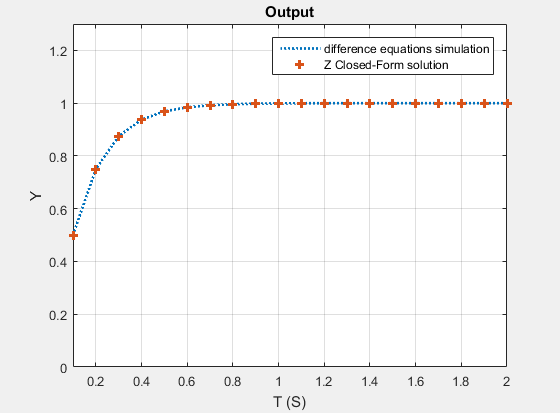
We can see from Fig. 1.3 that the filter output eventually matches the filter input. The amount of time it takes the filter output to reach 63% of its steady-state value is the filter time constant. Varying the filter gain G will change the time constant of the fading memory filter. We can also see from Fig. 1.3 that the simulation results agree with the closed-form solution.
从图1.3中可以看出滤波器的输出最终与滤波器的输入趋于一致。滤波器输出值达到稳态输出值63%时所用的时间称为滤波器的时间常数。通过改变增益G可以调整渐消记忆滤波器的时间常数。从图1.3中可以看出仿真结果与笔试解完全吻合。
REFERENCES 参考文献
[1] Selby, S. M., Standard Mathematical Tables—Twentieth Edition, Chemical Rubber Co., Cleveland, OH, 1972.
[2] Press, W. H., Flannery, B. P., Teukolsky, S. A., and Vetterling, W. T., Numerical Recipes: The Art of Scientific Computation, Cambridge Univ. Press, London, 1986.
[3] Schwarz, R., and Friedland, B., Linear Systems, McGraw-Hill, New York, 1965.


 3021
3021

 被折叠的 条评论
为什么被折叠?
被折叠的 条评论
为什么被折叠?
 到【灌水乐园】发言


