CHAPTER 2：Fundamentals of Tactical Missile Guidance 第二章：导弹制导原理

INTRODUCTION 引言

TACTICAL guided missiles apparently had their origin in Germany. For example, the Hs. 298 was one of a series of German air-to-air guided missiles developed by the Henschel Company during World War II [1]. A high-thrust first stage accelerated the missile from the carrier aircraft, whereas a low-thrust, long-burning sustainer maintained the vehicle’s velocity. The Hs. 298, which was radio controlled from the parent aircraft, was to be released either slightly above or below the target. Apparently the height differential made it easier to aim and guide the missile. This first air-to-air missile weighed 265 lb and had a range of nearly 3 miles. On December 22, 1944, three missiles were test flown from a JU88G aircraft. All three tests resulted in failure. Although 100 of these air-to-air missiles were manufactured, none was used in combat.

众所周知，战术导弹起源于德国。例如，在第二次世界大战期间亨舍尔公司研发的系列德国空空导弹中的[1]Hs.298就是其中之一。这型导弹采用大推力一级发动机实现导弹加速以脱离载机，之后采用小推力长燃烧时间的巡航级发动机维持导弹的飞行速度。Hs.298导弹采用载机无线电控制，允许在略高于或略低于目标的位置进行发射。显然，(载机与目标存在一定的) 高度差使载机更容易瞄准目标并实现对导弹的引导。第一枚空空导弹重265磅，射程接近3英里。1944年12月22日，三枚导弹分别挂载JU88G飞机开展了飞行试验，但三次试验都以失败告终。尽管此型空对空导弹共生产了100枚之多，但最终也没有一枚能用于实战。

The Rheintochter (R-1) was a surface-to-air missile also developed in Germany during World War II [1]. This unusual looking two-stage radio-controlled missile weighed nearly 4000 lb and had three sets of plywood fins: one for the booster and two for the sustainer. Eighty-two of these missiles flew before production was halted in December 1944. The missile was ineffective because Allied bombers, which were the R-1’s intended target, flew above the range (about 20,000 ft) of this surface-to-air missile.

Rheintocter（R-1）是德国在第二次世界大战期间研制的一种地对空导弹[1]。这枚外形独特采用两级推力方案的无线电制导导弹全重近4000磅。其配备有三套胶合板材质舵面：一套用于助推段控制，两套用于巡航级段控制。该型导弹在1944年12月停产之前已经有82枚完成了实弹飞行。但该导弹起到的作用却微乎其微，因为R-1主要打击目标盟军轰炸机的飞行高度通常都大于其射程（约20000英尺）。

Although proportional navigation was apparently known by the Germans during World War II at $Peenem\ddot{u}nde$, no applications on the Hs.298 or R-1 missiles using proportional navigation were reported [2]. The Lark missile, which had its first successful test in December 1950, was the first missile to use proportional navigation. Since that time proportional navigation guidance has been used in virtually all of the world’s tactical radar, infrared (IR), and television (TV) guided missiles [3]. The popularity of this interceptor guidance law is based upon its simplicity, effectiveness, and ease of implementation. Apparently, proportional navigation was first studied by C. Yuan and others at the RCA Laboratories during World War II under the auspices of the U.S. Navy [4].

尽管早在在二战期间，德国佩内明德（$Peenem\ddot{u}nde$）的科研人员们就已经掌握了比例导引的技术，但没有文献表明比例导引技术被应用在Hs.298 或 R-1 导弹上[2]。于1950年12月试验成功的Lark导弹，是有据可靠第一个使用比例导引的导弹。自此之后比例导引技术几乎被应用在了世界上所有的战术雷达、红外（IR）和电视制导导弹上[3]。这种拦截制导律具有简单、有效和易于实施等特点，因此深受导弹工程师的青睐。资料显示，第二次世界大战期间，在美国海军的支持下，RCA实验室的C.Yuan和其学者率先开展了对比例导引律的研究工作[4]。

The guidance law was conceived from physical reasoning and equipment available at that time. Proportional navigation was extensively studied at Hughes Aircraft Company [5] and implemented in a tactical missile using a pulsed radar system. Finally, proportional navigation was more fully developed at Raytheon and implemented in a tactical continuous wave radar homing missile [6]. After World War II, the U.S. work on proportional navigation was declassified and first appeared in the Journal of Applied Physics [7]. Mathematical derivations of the “optimality” of proportional navigation came more than 20 years later [8].

起初比例导引律是基于客观的物理规律和设备可操作性所构想出来的。休斯飞机公司[5]对比例导引律进行了广泛研究，并将其应用在的采用脉冲雷达体制的战术导弹上。随后，比例导引律在雷神公司得到了更全面的开发，并被应用在连续波雷达寻的战术导弹上[6]。第二次世界大战后，美国关于比例导引律的研究得以解密，并首次出现在《应用物理杂志》上[7]。而有关比例导引最优性的数学推论直到20年后才得以被证明[8]。

译者注：比例导引律从“好用”到“为什么好用”经历了近20年的时间，可见很多的技术创新都是伴随着工程应用而提出的，这些从实践中总结出的经验可能在短时间内缺少理论的支撑，但确是科技进步进程的重要推动力。

Keeping with the spirit of the origins of proportional navigation, we shall avoid mathematical proofs in this chapter on deriving the guidance law, but shall, instead, concentrate first on proving to the reader that the guidance technique works. Next we shall investigate some properties of the guidance law that we shall both observe and derive. Finally, we shall show how this classical guidance law provides the foundation for more advanced techniques of interceptor guidance.

秉承着比例导引律诞生的精神 。在本章中我们将不涉及制导律的数学推导过程，而着力于向读者证明制导技术的有效性。之后，我们将通过观察和推导的方式研究制导律的一些性质。最后，我们将说明为何比例导引这一经典制导律为被认为是更先进的拦截制导技术的基础。

译者注：译者认为这里所谓比例导引律的诞生精神，是指先使用后证明的实用主义精神

WHAT IS PROPORTIONAL NAVIGATION? 什么是比例导引?

Theoretically, the proportional navigation guidance law issues acceleration commands, perpendicular to the instantaneous missile-target line-of-sight, which are proportional to the line-of-sight rate and closing velocity. Mathematically, the guidance law can be stated as.

理论上，比例导引律用于生成垂直于瞬时弹目连线方向上的加速度指令，这个加速度指令与视线角速度和抵近速度成正比。比例导引律的数学表达式为

$$n_c=N^{\prime }{V}_c\dot{\lambda }$$

译者注：使用 $N^{\prime }{V}_c\dot{\lambda }$ 所得加速度指令，本书采用英制单位，为ft/s/s（使用公制单位为m/s/s），其中 $\dot{\lambda }$ 的单位为rad/s（或/s）, N‘ 为无量纲数 。

译者注：所谓“视线”就是“导弹与目标的连线”（也称“弹-目视线“、”弹目连线“、”瞄准线“等）。将导弹的导引头理解成一双“眼睛”，这双导弹的眼睛可以始终紧盯目标，因此导弹与目标的连线就如同视觉形成的线一样，所以称为“视线”。可见，视线只与导弹和目标的位置有关，导弹或者目标的位置发生变化，则视线才会变化，与导弹和目标的姿态无关。

where $n_c$ is the acceleration command (in $ft/s^2$ ), N’ a unitless designer-chosen gain (usually in the range of 3–5) known as the effective navigation ratio, $V_c$ the missile-target closing velocity (in $ft/s$), and l the line-of-sight angle (in rad). The overdot indicates the time derivative of the line-of-sight angle or the line-of-sight rate.

其中$n_c$是加速度指令（单位：$ft/s^2$），$N^{\prime }$是设计者选择的无量纲增益，称为有效导引比（通常在3~5的范围内），$V_c$是导弹抵近目标的速度（单位：$ft/s$），$\lambda$是视线角（单位：$rad$）。表达式的上标一点表示视线角或视线速率的时间导数。

In tactical radar homing missiles using proportional navigation guidance, the seeker provides an effective measurement of the line-of-sight rate, and a Doppler radar provides closing velocity information. In tactical IR missile applications of proportional navigation guidance, the line-of-sight rate is measured, whereas the closing velocity, required by the guidance law, is “guesstimated.”

在使用比例导引律的雷达制导战术导弹中，导引头可提供视线角速度的有效测量量，多普勒雷达提供抵近目标的速度信息。在使用比例导引律的红外导引战术导弹中，视线角速率是实际测量量，而制导律中所用的抵近速度是“估计值”。

译者注：红外、电视、被动雷达等被动导引头无法提供弹目相对距离、速度信息，因此在使用比例导引过程中需要对抵近速度进行估计。

In tactical endoatmospheric missiles, proportional navigation guidance commands are usually implemented by moving fins or other control surfaces to obtain the required lift. Exoatmospheric strategic interceptors use thrust vector control, lateral divert engines, or squibs to achieve the desired acceleration levels.

对于在大气层内飞行的战术导弹而言，主要通过偏转气动舵面或其他控制面的方式获得气动升力，用于提供实现比例导引律所需的加速度。而对于在大气层外飞行的战略拦截导弹，主要使用推力矢量控制、直接侧向力控制或矢量发动机等装置来提供导弹所需的加速度。

译者注：对于要飞出大气层，且在大气层外仍然需要进行机动的导弹通常都用于拦截导弹的防空导弹，即所谓的“反导导弹”，英语中称为interceptor即拦截器

SIMULATION OF PROPORTIONAL NAVIGATION IN TWO DIMENSIONS 二维空间比例导引仿真

To better understand how proportional navigation works, let us consider the two-dimensional, point mass missile-target engagement geometry of Fig. 2.1. Here we have an inertial coordinate system fixed to the surface of a flat-Earth model (that
is, the 1 axis is downrange and the 2 axis can either be altitude or crossrange).Using the inertial coordinate system of Fig. 2.1 means that we can integrate components of the accelerations and velocities along the 1 and 2 directions without having to worry about additional terms due to the Coriolis effect. In this model it is assumed that both the missile and target travel at constant velocity. In addition, gravitational and drag effects have been neglected for simplicity.

为了更好地理解比例导引率的工作原理，让我们以图2.1中的二维空间内的质点弹-目交战几何模型为例来进行分析。图中有一个固定在平面地球模型表面的惯性坐标系（1轴为射向方向，2轴可以是高度方向或横向方向）。使用如图2.1中的惯性坐标系意味着我们可以沿1和2方向的进行加速度和速度分量的积分，而不必考虑科里奥利效应带来的附加项。该模型中，假设导弹和目标都以恒定速度飞行，且为了简单起见，已忽略了重力和阻力作用。

译者注：牛顿第二定律只有在惯性坐标系中才成立，否则需要在公式中进行牵连加速度补偿，而科里奥利效应就是由于地球旋转，不能视为惯性坐标系而引入的补偿量。

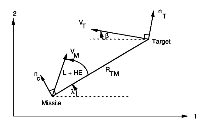Fig. 2.1 Two-dimensional missile-target engagement geometry. 图2.1 二维空间中的弹目交战几何模型

We can see from the figure that the missile, with velocity magnitude $V_M$ , is heading at an angle of $L+HE$ with respect to the line of sight. The angle $L$ is known as the missile lead angle. The lead angle is the theoretically correct angle for the missile to be on a collision triangle with the target. In other words, if the missile is on a collision triangle, no further acceleration commands are required for the missile to hit the target. The angle $HE$ is known as the heading error. This angle represents the initial deviation of the missile from the collision triangle.

从图中可以看出，导弹以$V_M$的速率飞行，速度方向与视线方向 ( 弹目连线方向 ) 的夹角为$L+HE$。角度$L$被称为导弹前置角。如果导弹与视线夹角为$L$的方向飞行，则理论上导弹、目标和航迹交汇点将构成一个碰撞三角形。换句话说，如果导弹位于碰撞三角形中，则在导弹不需要进行任何的机动就可以直接命中目标。角$HE$被称为航向偏差角，这个角度表示初始条件下导弹速度方向与可构成碰撞三角形的理想速度方向之间的偏差。

译者注： 如果导弹和目标都进行匀速直线运动，则理论上必然存在一个方向，使得当导弹沿该方向飞行时，刚好可以在抵达航迹的交点时命中目标。这个理想的飞行方向理论上是存在的，且不是导弹-目标的视线方向，而是要在视线方向基础上向目标运动前方留有一定的角度提前量（因为在抵近过程中目标也在运动），这个角度提前量就称为导弹前置角。航向偏差角可视为初始时刻导弹速度方向与理想速度方向之间的偏差。

译者注：heading error表示初始时刻导弹实际速度方向与可构成碰撞三角形的理想速度方向之间的偏差，这里的heading表示速度矢量的方向，并不单指水平面内的狭义航向，也可以指纵向平面内速度矢量方向。

In Fig. 2.1 the imaginary line connecting the missile and target is known as the line of sight. The line of sight makes an angle of $\lambda$ with respect to the fixed reference, and the length of the line of sight (instantaneous separation between missile and target) is a range denoted $R_{TM}$ . From a guidance point of view, we desire to make the range between missile and target at the expected intercept time as small as possible (hopefully zero). The point of closest approach of the missile and target is known as the miss distance.

图2.1中，连接导弹和目标的假想连线称为视线。视线与固定坐标轴之间的夹角为$\lambda$，视线长度（导弹和目标之间的实时距离）为$R_{TM}$。从制导角度来看，我们希望在预期的拦截时间内使导弹和目标之间的距离尽可能小（最好为零）。导弹与目标最接近时的弹目距离称为脱靶量。

The closing velocity $V_c$ is defined as the negative rate of change of the distance from the missile to the target, or

抵近速度$V_c$定义为弹目距离变化率的相反数，或

$$V_c=-{\dot{R}}_{TM}$$

译者注：需要注意的是导引律中涉及到的速度为弹目的相对运动速度（翻译为抵近速度），并非导弹自身的速度。但如果是对静止目标或者慢速目标进行打击时，可以近似为导弹速度。从其定义来看当弹目距离缩小时速度为正。

Therefore, at the end of the engagement, when the missile and target are in closest proximity, the sign of $V_c$ will change. In other words, from calculus we know that the closing velocity will be zero when $R_{TM}$ is a minimum (that is, the function is either minimum or maximum when its derivative is zero). The desired acceleration command $n_c$ , which is derived from the proportional navigation guidance law, is perpendicular to the instantaneous line of sight.

因此，在交战过程末段，当导弹和目标距离最接近时，$V_c$的符号将发生变化。换言之，根据微积分原理，当抵近速度将变为零时（即导数为零时，原函数取到极值）$R_{TM}$取到最小值时。比例导引制导律所得期望加速度指令$n_c$始终垂直于弹目视线。

In our engagement model of Fig. 2.1, the target can maneuver evasively with acceleration magnitude $n_T$ . Since target acceleration $n_T$ in the preceding model is perpendicular to the target velocity vector, the angular velocity of the target can be expressed as
在图2.1所示的交战模型中，目标能够以$n_T$的加速度进行躲避机动。模型中目标加速度$n_T$始终垂直于目标速度矢量，因此目标的方位角速度可以表示为：
$$\dot{\beta }=\frac{n_T}{V_T}$$

译者注：$\dot{\beta }$的单位为rad/s，$n_T$表示加速度（单位ft/s/s）而非过载（单位g）。

译者注：作为被攻击对象，目标在发现自身处于危险时或者进行突防时会进行规避性的机动，通常目标机动的目的是为导弹创造“麻烦”，已达到增加导弹的脱靶量或者逃离导弹的跟踪范围的目的，而不会依据弹目信息进行“最优规避”机动，也通常不会进行加减速机动。因此将目标的加速度定义为垂直于自身速度方向是合理的，且从后续的研究来看，目标沿垂直于速度的方向机动对于导弹而言是最严酷的情况。

where $V_T$ is the magnitude of the target velocity. The components of the target velocity vector in the Earth or inertial coordinate system can be found by integrating the differential equation given earlier for the flight-path angle of the target $\dot{\beta }$ and substituting in

其中$V_T$表示目标速度的大小。目标速度矢量在地球坐标系（或称为惯性坐标系）中的投影分量可以通过微分方程积分得到。在给定目标弹道角度$\beta$的前提下，将目标速度$V_T$带入下式得

$$V_{T1}=-V_{T}cos\beta$$
$$V_{T2}=V_{T}sin\beta$$

Target position components in the Earth fixed coordinate system can be found by directly integrating the target velocity components. Therefore, the differential equations for the components of the target position are given by

目标位置在地球坐标系（或称为惯性坐标系）中的投影分量可直接对目标速度进行积分获得。因此，目标位置分量的微分方程为

$${\dot{R}}_{T1}=V_{T1}$$
$${\dot{R}}_{T2}=V_{T2}$$

Similarly, the missile velocity and position differential equations are given by
同理，导弹的速度和位置微分方程为：

$${\dot{V}}_{M1}=a_{M1}$$
$${\dot{V}}_{M2}=a_{M2}$$
$${\dot{R}}_{M1}=V_{M1}$$
$${\dot{R}}_{M2}=V_{M2}$$

where a M1 and a M2 are the missile acceleration components in the Earth coordinate system. To find the missile acceleration components, we must first find the components of the relative missile-target separation. This is accomplished by first defining the components of the relative missile-target separations by

其中$M1$和$M2$是导弹加速度在地球坐标系中的分量。为了得到导弹加速度分量，我们必须首先求取导弹相对于目标的距离分量。首先定义导弹目标相对距离：

$$R_{TM1}=R_{T1}-R_{M1}$$
$$R_{TM2}=R_{T2}-R_{M2}$$

We can see from Fig. 2.1 that the line-of-sight angle can be found, using trigonometry, in terms of the relative separation components as
如图2.1所示，可使用三角几何关系，根据弹目距离在两坐标轴上的分量，求取视线角$\lambda$。

$$\lambda =ta{n}^{-1}\frac{R_{TM2}}{R_{TM1}}$$

If we define the relative velocity components in Earth coordinates to be
如果定义相对速度在地球坐标系上的投影分量为

$$V_{TM1}=V_{T1}-V_{M1}$$
$$V_{TM2}=V_{T2}-V_{M2}$$

we can calculate the line-of-sight rate by direct differentiation of the expression for line-of-sight angle. After some algebra we obtain the expression for the line-of-sight rate to be
则直接对视线角表达式求导可得到视线角速率。经过若干几何运算后，所得视线角速率的表达式为

$$\dot{\lambda }=\frac{R_{TM1}{V}_{TM2}-R_{TM2}{V}_{TM1}}{R_{RM}^2}$$

译者注：表达式中可以看出，弹目视线角和弹目视线角速率仅与弹目的相对运动有关。与其绝对运动并不直接相关。

The relative separation between missile and target $R_{TM}$ can be expressed in terms of its inertial components by application of the distance formula, as
根据弹目距离在惯性系上的投影分量，利用距离计算公式，可以得到弹目相对距离的表达式为

$$R_{TM}=(R_{TM1}^2+R_{TM2}^2{)}^{\frac{1}{2}}$$

Because the closing velocity is defined as the negative rate of change of the missile target separation, it can be obtained by differentiating the preceding equation, yielding
由于抵近速度定义为弹目相对距离变化率的相反数，因此将上式求导后可以得到

$$V_c=-{\dot{R}}_{TM}=\frac{-(R_{TM1}{V}_{TM1}+R_{TM2}{V}_{TM2})}{R_{TM}}$$

The magnitude of the missile guidance command $n_c$ can then be found from the definition of proportional navigation, or

则根据比例导引法的定义，导弹过载指令大小$n_c$为

$$n_c=N^{\prime }{V}_c\dot{\lambda }$$

Because the acceleration command is perpendicular to the instantaneous line of sight, the missile acceleration components in Earth coordinates can be found by trigonometry using the angular definitions from Fig. 2.1. The missile acceleration components are
由于加速度指令实时垂直于弹目视线，结合图2.1中定义的角速度，使用几何三角关系，可求出导弹加速度在地球坐标系上的分量。导弹加速度分量可表示为：

$$a_{M1}=-n_{c}sin\lambda$$
$$a_{M2}=n_{c}cos\lambda$$

We have now listed all of the differential equations required to model a complete missile-target engagement in two dimensions. However, some additional equations are required for the initial conditions on the differential equations in order to complete the engagement model.
到目前为止，本文已给出了用于构建二维平面弹目交战模型所需的所有微分方程。然而为了完成交战过程的建模，还需要提供几个额外的方程用于微分方程初始化。

A missile employing proportional navigation guidance is not fired at the target but is fired in a direction to lead the target. The initial angle of the missile velocity vector with respect to the line of sight is known as the missile lead angle $L$. In essence we are firing the missile at the expected intercept point. We can see from Fig. 2.1 that, for the missile to be on a collision triangle (missile will hit the target if both continue to fly along a straight-line path at constant velocities), the theoretical missile lead angle can be found by application of the law of sines, yielding
使用比例导引的导弹不应正对着目标发射，而是领先于目标运动前方发射。初始时刻导弹的速度方向与视线方向之间的夹角称为前置角$L$。实际上，我们会冲着期望的弹目交汇点发射导弹。从图2.1中可以看出，如果导弹处在碰撞三角形中（即如果导弹和目标都继续做匀速直线运动则导弹将直接集中目标），则可以根据三角函数原理求取导弹的理论前置角。

$$L=si{n}^{-1}\frac{V_{T}sin(\beta +\lambda )}{V_M}$$

In practice, the missile is usually not launched exactly on a collision triangle, as the expected intercept point is not known precisely. The location of the intercept point can only be approximated because we do not know in advance what the target will do in the future. In fact, that is why a guidance system is required ! Any initial angular deviation of the missile from the collision triangle is known as a heading error $HE$. The initial missile velocity components can therefore be expressed in terms of the theoretical lead angle $L$ and actual heading error $HE$ as
工程实现上，准确的命中点是未知的，因此导弹在发射时不可能正好满足碰撞三角形条件，且由于我们不能提前预测目标的行为，因此只能对命中点进行大致的估计。事实上，这也是我们为什么需要导引律的原因！初始时刻任何使得导弹偏离碰撞三角形的初始角度偏差统称为航向误差角$HE$。据此，初始导弹速度分量可以用理论前置角$L$和实际航向误差角$HE$表示为

$$V_{M1}(0)=V_{M}cos(L+HE+\lambda )$$
$$V_{M2}(0)=V_{M}sin(L+HE+\lambda )$$

TWO-DIMENSIONAL ENGAGEMENT SIMULATION 二维平面交战仿真

To witness and understand the effectiveness of proportional navigation, it is best to simulate the guidance law and test its properties under a variety of circumstances. A two-dimensional missile-target engagement simulation was set up using the differential equations derived in the previous section. The simulation inputs are the initial location of the missile and target, speeds, flight time, and effective navigation ratio. The user can vary the level of the two error sources considered: target maneuver and heading error.
为了说明并解释比例导引的有效性，最好构建一个比例导引的仿真环境，并在不同的情景下对其进行测试。本节使用前一小节得到的微分方程组，构建出一个二维平面内的弹目交战仿真模型。仿真模型的输入为导弹和目标的初始位置，速度，飞行时间以及有效导引系数。用户可以对模型中的两个误差源，目标机动和航向误差，进行配置。

LISTING 2.1 TWO-DIMENSIONAL TACTICAL MISSILE-TARGET ENGAGEMENT SIMULATION
表2.1 二维平面战术导弹-目标交战模型仿真

n=0;

% 状态量初始化
VM = 3000.;     % 导弹速度
VT = 1000.;     % 目标速度
XNT = 0.;       % 目标加速度
HEDEG = -20.;   % 航向误差角（度）
XNP = 4.;       % 有效比例导引系数
RM1 = 0.;       % 导弹初始位置
RM2 = 10000.;
RT1 = 40000.;   % 目标初始位置
RT2 = 10000.;
BETA=0.;        % 目标初值速度方向
VT1=-VT*cos(BETA);  % 目标初始速度
VT2=VT*sin(BETA);

HE=HEDEG/57.3;      % 误差角（弧度）
T=0.;               % 时标
S=0.;               % 数据记录时标

% 弹目初始相对状态量计算
RTM1=RT1-RM1;       %  弹目距离 
RTM2=RT2-RM2;       %  
RTM=sqrt(RTM1*RTM1+RTM2*RTM2);
XLAM=atan2(RTM2,RTM1);              % 弹目视线角
XLEAD=asin(VT*sin(BETA+XLAM)/VM);   % 初始前置角
THET=XLAM+XLEAD;                    % 初始速度偏角
VM1=VM*cos(THET+HE);                % 初始速度
VM2=VM*sin(THET+HE);
VTM1 = VT1 - VM1;                   % 弹目相对速度
VTM2 = VT2 - VM2;
VC=-(RTM1*VTM1 + RTM2*VTM2)/RTM;    % 抵近速度

%% 非线性弹目关系仿真
while VC >= 0       % 命中前
    % 设定仿真步长
    if RTM < 1000   
        H=.0002;
    else
        H=.01;
    end
    
    % 记录状态量旧值
    BETAOLD=BETA;
    RT1OLD=RT1;
    RT2OLD=RT2;
    RM1OLD=RM1;
    RM2OLD=RM2;
    VM1OLD=VM1;
    VM2OLD=VM2;
    
    STEP=1;
    FLAG=0;
    while STEP <=1
        if FLAG==1
            STEP=2;
            %单步状态量预测
            BETA=BETA+H*BETAD;
            RT1=RT1+H*VT1;
            RT2=RT2+H*VT2;
            RM1=RM1+H*VM1;
            RM2=RM2+H*VM2;
            VM1=VM1+H*AM1;
            VM2=VM2+H*AM2;
            % 仿真时间更新
            T=T+H;
        end
        
        % 弹目相对值计算
        RTM1=RT1-RM1;           % 弹目相对位置
        RTM2=RT2-RM2;
        RTM=sqrt(RTM1*RTM1+RTM2*RTM2);
        VTM1=VT1-VM1;           % 弹目相对速度
        VTM2=VT2-VM2;
        VC=-(RTM1*VTM1+RTM2*VTM2)/RTM;
        
        XLAM=atan2(RTM2,RTM1);  % 弹目视线角
        XLAMD=(RTM1*VTM2-RTM2*VTM1)/(RTM*RTM);  % 弹目视线角速度
        XNC=XNP*VC*XLAMD;       % NVQ_ 比例导引得到加速度指令
        AM1=-XNC*sin(XLAM);     % 导弹加速度
        AM2=XNC*cos(XLAM);
        VT1=-VT*cos(BETA);      % 目标速度
        VT2=VT*sin(BETA);
        BETAD=XNT/VT;           % 目标速度偏角
        FLAG=1;
    end
    FLAG=0;
    
    % 使用二阶龙格库塔法更新状态量
    BETA=.5*(BETAOLD+BETA+H*BETAD);
    RT1=.5*(RT1OLD+RT1+H*VT1);
    RT2=.5*(RT2OLD+RT2+H*VT2);
    RM1=.5*(RM1OLD+RM1+H*VM1);
    RM2=.5*(RM2OLD+RM2+H*VM2);
    VM1=.5*(VM1OLD+VM1+H*AM1);
    VM2=.5*(VM2OLD+VM2+H*AM2);
    
    % 状态量记录
    S=S+H;
    if S >=.09999
        S=0.;
        n=n+1;
        ArrayT(n)=T;
        ArrayRT1(n)=RT1;
        ArrayRT2(n)=RT2;
        ArrayRM1(n)=RM1;
        ArrayRM2(n)=RM2;
        ArrayXNCG(n)=XNC/32.2;
        ArrayRTM(n)=RTM;
    end
end
RTM

%% 图像绘制
figure
plot(ArrayRT1,ArrayRT2,ArrayRM1,ArrayRM2),grid
title('Two-dimensional tactical missile-target engagement simulation')
xlabel('Downrange (Ft) ')
ylabel('Altitude (Ft)')

figure
plot(ArrayT,ArrayXNCG),grid
title('Two-dimensional tactical missile-target engagement simulation')
xlabel('Time (sec)')
ylabel('Acceleration of missle (G)')

%% 数据存储
clc
output=[ArrayT',ArrayRT1',ArrayRT2',ArrayRM1',ArrayRM2',ArrayXNCG',ArrayRTM' ];
save datfil.txt output -ascii
disp '*** Simulation Complete'

A tactical missile-target engagement simulation appears in Listing 2.1. We can see from the listing that the missile and target differential equations are solved using the second-order Runge–Kutta numerical integration technique. As was the case in the second-order system simulation of Chapter 1, the differential equations appear before the FLAG=1 statement. The integration step size is fixed for most of the flight ($H=0.01s$) but is made smaller near the end of the flight ($H=0.0002s$ when $R_{TM}<1000ft$) to accurately capture the magnitude of the miss distance.

表2.1给出了一个战术导弹-目标交战仿真模型代码。从表中可以看出，程序使用了二阶Runge–Kutta数值积分法求解弹目微分方程。与第一章中二阶系统的仿真程序类似，FLAG=1语句的上一行语句为微分方程表达式。在大部分飞行阶段中，积分步长为一固定值($H=0.01s$) ，而在飞行末段会采用更小的积分步长 ($H=0.0002s$ when $R_{TM}<1000ft$)以便提升脱靶量的计算精度。

The program is terminated when the closing velocity changes sign, because this means that the separation between the missile and target is a minimum. At this time the missile-target separation is the miss distance: We can see from the preceding equations that the miss distance will always be positive because it is calculated from the distance formula. We can see from the listing that errors can be introduced by changing values in the data statements. Status of the missile and target location, along with acceleration and separation information, is displayed every 0.1s. Note that the missile acceleration is written to a file datfil.txt in units of gravity.
当抵近速度反号时终止仿真程序，因为反号意味着弹目距离已达到最小值，且这时的弹目距离就是所谓的脱靶量。从上文所述的方程中可以看出：由于脱靶量是使用距离公式计算的，因此脱靶量的值始终大于零。从程序中可以看出，通过更改数据状态的方式可选择是否引入误差。程序每隔0.1s对导弹状态、目标位置以及加速度和弹目距离数据进行记录。请注意，导弹的加速度数据（单位已折算为g）被保存在名为datfil.txt文件中。

译者注：这里存储的加速度数据单位为g（在存储时除转换为了g）

Fig. 2.2 Increasing effective navigation ratio causes heading error to be removed more rapidly
图 2.2 增大有效比例导引系数可以更快的消除导弹的航向误差

A sample case was run in which the only disturbance was a 20-deg heading error ( $HEDEG=–20$ ). Sample trajectories for effective navigation ratios of 4 and 5 are depicted in Fig. 2.2. We can see from the figure that initially the missile is flying in the wrong direction because of the heading error. Gradually the guidance law forces the missile to home on the target. The larger effective navigation ratio enables the missile to remove the initial heading error more rapidly, thus causing a much tighter trajectory. In both cases, proportional navigation appears to be an effective guidance law because the missile hits the target (near zero miss distance with the simulation).

对仅引入-20°( $HEDEG=–20$ )航向误差的简单场景进行仿真。图2.2 中绘制了当有效导引系数为4和5时的航迹采样结果。从图中可以看出，由于航向误差的存在 (起初) 导弹向着错误的方向飞行。(之后) 制导律逐步迫使导弹导向目标。更大的有效导引系数可以更快的消除导弹的航向误差，因此“更大”的导引系数在图中形成了一个“更高”的航迹曲线。在所示两种场景中导弹均可命中目标（仿真结果显示，脱靶量接近于0），由此可见比例导引是一种非常有效的导引规律。

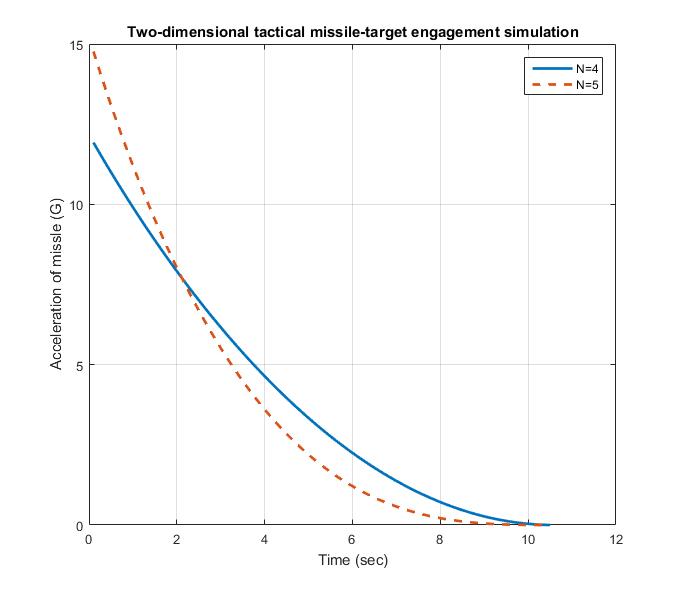
Fig. 2.3 Increasing effective navigation ratio causes more acceleration initially.
图2.3增大有效比例导引系数会提升制导初段的加速度

The resultant missile acceleration histories, displayed in Fig. 2.3, for both cases are somewhat different. The quicker removal of heading error in the higher effective navigation ratio case ($N^{\prime }=5$) results in larger missile accelerations at the beginning of the flight and lower accelerations near the end of the flight. In both cases the acceleration profiles for the required missile acceleration to take out the heading error and to hit the target is monotonically decreasing and zero at the end of the flight. Thus, a property of a proportional navigation guidance system is to start taking out heading error as soon as possible but also gradually throughout the entire flight. In Chapter 15 we shall study a guidance system that tries to remove the entire heading error immediately. By increasing the effective navigation ratio, we are allowing the missile to take out heading error more rapidly.
如图2.3所示，(有效导引系数为4和5) 两种情况下导弹加速度数据有所不同。选取较大有效导引系数的情况($N^{\prime }=5$)下 ，航向误差的快速消除，导致弹道初段导弹加速度较大，而在弹道末段的加速度较小。在不同导引参数下，用于消除航向误差实现目标打击的所需的加速度随时间单调递减，且在弹道末段减小到0。因此，比例导航制导系统的一个特点是：在进入制导流程后立即开始消除航向误差，但误差消除过程贯穿后续的飞行过程始终。在第15章中，我们将研究一种力求即刻消除全部航向误差的制导系统。通过提高有效导引比的方式，可以加快导弹消除航向误差的速度。

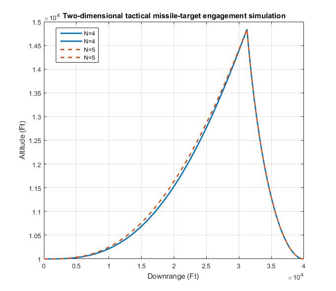
Fig. 2.4 Proportional navigation works against maneuvering target
图2.4 使用比例导引法对抗机动目标

Another sample case was run in which the only disturbance was a 3-g target maneuver ( $XNT=96.6,HEDEG=0$). In this scenario the missile and target are initially on a collision triangle and flying along the downrange component of the Earth fixed coordinate system (cross-range velocity components of both interceptor and target are zero). Therefore, the target velocity vector is initially along the line of sight, and at first all 3 g of the target acceleration are perpendicular to the line of sight. As the target maneuvers, the magnitude of the target acceleration perpendicular to the line of sight diminishes due to the turning of the target. Sample missile-target trajectories for this case with effective navigation ratios of 4 and 5 are depicted in Fig. 2.4. We can see that the higher effective navigation ratio causes the missile to lead the target slightly more than the lower navigation ratio case. Otherwise the trajectories are virtually identical. In both cases, the proportional navigation guidance law enabled the missile to hit the maneuvering target.

在另一个简单场景的仿真中，仅引入3g( $XNT=96.6,HEDEG=0$ )目标机动干扰。在该场景中，导弹和目标在初始时刻就处在碰撞三角形中，并沿着地球坐标系横轴方向飞行（导弹和目标速度的横向分量均为0）。在初始时刻，目标的速度向量沿着视线方向，3g的目标加速度垂直于视线方向。随着目标机动，目标不断进行转向，目标加速度垂直于视线方向的分量逐步减小。图2.4显示了有效导引系数分别为4和5时航迹的采样结果。可见更大的有效导引系数可略微提升导弹的引导能力。除此之外，两者的航迹从视觉上来看较为类似。对于所示两种场景，比例导引律均可以引导导弹命中机动目标。

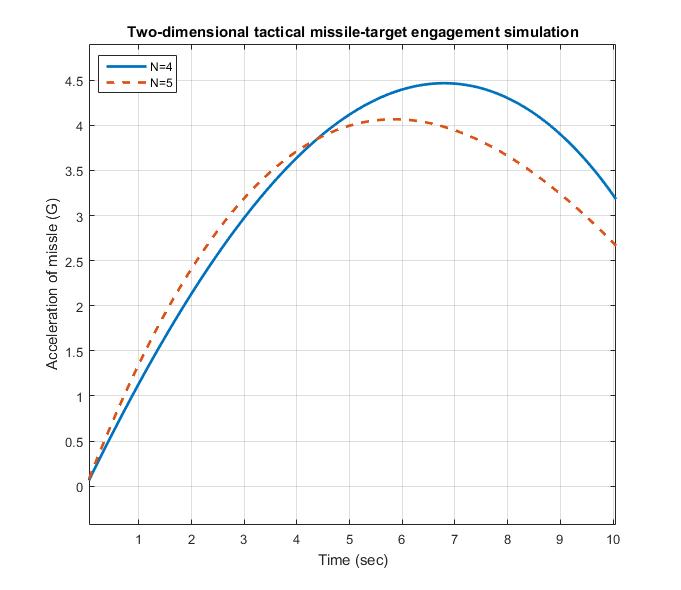Fig. 2.5 Higher navigation ratio yields less acceleration to hit maneuvering target. 图2.5 更高的比例导引系数会降低命中目标的的加速度来命中机动目标。

However, Fig. 2.5 shows that there are significant differences between the acceleration profiles for the maneuvering target case. Although both acceleration profiles are virtually monotonically increasing for the entire flight, the higher effective navigation ratio requires less acceleration capability of the missile. In addition, we can see that the peak acceleration required by the missile to hit the target is significantly higher than the maneuver level of the target (3 g).
然而图2.5却表明，对于目标机动场景有效导引系数的不同所对应的加速度剖面有着明显的差别。虽然从视觉上来看，不同系数对应的加速度剖面在整个飞行过程中均随时间的增长而变大，但较大的有效导引系数对导弹的最大加速度需求更小。另外，值得注意的是，为了命中目标导弹的最大加速度需求要远远大于目标的加速度能力（3g）。

译者注：原文中在描述加速度变化趋势时使用了 monotonically increasing 直接翻译为单调递增，但是从图像来看，加速度曲线并非单调递增，而是在某个时刻达到最大值。结合后文中线性化后加速度曲线的仿真结果为单调递增的现象推测作者的只是想强调在应对目标机动时加速度随时间增长这一事实，以区别于在应对航向误差时导弹加速度随时间递减的现象。

In both simulation examples we have seen the effectiveness of proportional navigation guidance. First we saw that proportional navigation is able to hit a target, even if it is initially launched in the wrong direction by 20 deg. Then we observed that the guidance law was also effective in hitting a maneuvering target. In both cases certain acceleration levels were required of the missile in order for it to hit the target. The levels were dependent on the type of error source and the effective navigation ratio. If the missile does not have the acceleration required by the guidance law, a miss will result.

通过述两个案例我们可以体会到比例导引法的有效性。首先我们见证了，即使在初始航向误差角达到20°时，比例导引法也可以引导导弹命中目标。之后我们观察到比例导引法在对机动目标的打击场景中依然有效。在两个场景中，为了使导弹命中目标，要求导弹具备一定的机动能力。而机动能力需求与误差源种类和有效导引比有关。如果导弹无法提供制导律所需加速度的大小，则会出现命中偏差。

译者注： 当导弹与目标正好处于碰撞三角形中时视线角速度为0，导弹无需采取任何机动。当导弹飞行方向偏离理论碰撞点，则会产生一定的视线角速度，在不对导弹进行引导的条件下弹目距离越近，产生的视线角速率越大。

译者注：在众多的状态量中，作者唯独列举了“加速度”的变化曲线，也暗示了在制导流程中加速度是导弹设计需求中非常重要的一个指标。从原理来看，制导流程属于“弹道控制”层面（即研究在给定弹目相对运动关系的前提下研究导弹的轨迹如何变化），而实现弹道控制的直接“手段”就是加速度。

译者注：从仿真结果看，如果被打击目标为匀速直线运动目标，则选取较小的N’有助于降低导弹加速度需求；而如果被打击目标为机动目标则选取较大的N’有助于降低导弹加速度需求。

译者注： 有效比例导引系数 N’ 决定相同的视线角速度所产生加速度指令的大小。选取比较大的 N’ 则在较小的角速度下导弹也会产生较大的加速度指令，“提前”消除导航误差，对于机动目标而言较大的 N’ 避免目标机动在导引段后期引起的更大的偏差，这就是为何较大的 N’ 可以降低加速度需求的原因。

LINEARIZATION 线性化

Thus far our understanding of the effectiveness of proportional navigation has come from the numerical simulation results of the two-dimensional engagement simulation. It is critical for the analysis, understanding, and development of design relationships to temporarily depart from the nonlinear missile-target simulation and develop a simpler model. Therefore, we will linearize the two-dimensional engagement model in the hope of gaining more understanding. This does not mean that we will abandon the nonlinear engagement model. In fact, we will always use the nonlinear engagement model to verify the insights generated by powerful analytical techniques to be used on the linearized engagement model.

到现在为止，我们对比例导引有效性的理解都是来自于二维平面交战模型的数值仿真结果。为了更好地分析、理解和研究弹目相对运动关系，需要暂时将非线性弹目仿真放在一边，并提出一个跟简单的模型。因此为了加深理解，我们将对二维平面的交战模型进行线性化。然而，这并不意味着我们会放弃非线性交战模型，实际上，我们将不断使用非线性交战模型来验证那些利用线性模型强大分析技术所得出的结论。

译者注：此处的relationships译者认为翻译成“弹目相对运动关系”较为贴切。制导的本质就是研究弹目相对运动关系。

The linearization of the missile-target geometry can easily be accomplished if we define some new relative quantities as shown in Fig. 2.6. Here $y$ is the relative separation between the missile and target perpendicular to the fixed reference.

如图2.6所示，若我们定义一些新的相对量，便很容易实现导弹-目标几何关系的线性化。这里$y$是弹目相对距离垂直于坐标轴的分量。

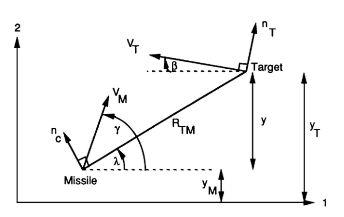
Fig. 2.6 Engagement model for linearization.
图 2.6 交战模型线性化

The relative acceleration (difference between missile and target acceleration) can be written by inspection of Fig. 2.6 as
从图2.6可以看出，相对加速度（导弹和目标加速度之差）可写成

$$\ddot{y}=n_{T}cos\beta -n_{c}cos\lambda$$

If the flight-path angles are small (near head-on or tail chase case), the cosine terms are approximately unity, and the preceding equation becomes
如果飞行航迹角很小（比较接近迎面或尾追的情况），则余弦项可近似为1，上述方程变为

$$\ddot{y}=n_T-n_c$$

Similarly, the expression for the line-of-sight angle can also be linearized using the small-angle approximation, yielding
类似地，视线角的表达式也可以使用小角度近似假设进行线性化

$$\lambda =y/R_{TM}$$

For a head-on case, we can approximate the closing velocity as
对于迎面情况，我们可以将抵近速度近似为

$$V_c=V_M+V_T$$

whereas in a tail chase case, the closing velocity can be approximated as
而在尾追情况下，抵近速度可以近似为

$$V_c=V_M-V_T$$

Therefore, in a linearized analysis we will treat the closing velocity as a positive constant. Because closing velocity has also been previously defined as the negative derivative of the range from the missile to target, and since the range must go to zero at the end of the flight, we can also linearize the range equation with the time-varying relationship
在线性化分析中，我们将抵近速度视为一个正常数。而上文中抵近速度被定义为弹目距离的负导数，且在飞行结束时弹目距离必为零，因此我们也可以将弹目距离方程线性化为如下的时变函数

$$R_{TM}=V_c(t_F-t)$$

where $t$ is current time and $t_F$ the total flight time of the engagement. Note that $t_F$ is also now a constant. The quantity $t_F–t$ is the time to go until the end of the flight. Therefore, the range from the missile to the target is also the closing velocity multiplied by the time to go until intercept. Because range goes to zero at the end of the flight by definition, we must reexamine the definition of miss distance. The linearized miss distance is taken to be the relative separation between missile and target y at the end of the flight, or
其中$t$是当前时刻，$t_F$是交战过程的总飞行时间。注意，$t_F$目前被当做一个常量。变量 $t_F–t$ 表示剩余飞行时间。因此弹目距离也可表示为抵近速度乘以剩余飞行时间。根据定义，飞行结束时弹目距离为零，所以我们必须重新考量脱靶量的定义。线性化后的脱靶量定义为飞行结束时导弹和目标之间的相对距离（$y$），即

$$Miss=y(t_f)$$

Because the linearized miss is not obtained from the distance formula, it is only an approximation to the actual miss. However, we shall soon see that the miss distance approximation is very accurate.
线性化后脱靶不是由距离公式计算所得，因此它只是实际脱靶的近似值。但我们很快就会发现脱靶距离近似值非常精确。

LINEARIZED ENGAGEMENT SIMULATION 线性交战模型仿真

In the previous section we developed linearized equations for the missile-target engagement. In this section we will see if the resultant linearized equations give performance projections that have trends similar to those of the nonlinear engagement equations. If they do not, then there is no point in developing design relationships based on a meaningless model. If they do, then there may be a point for the interested reader to continue reading this text!
在上一节中，我们研究了弹目交战的线性化方程。在本节中，我们将会了解利用线性化方程与非线性交战方程对性能的预测具是否具有相似的趋势。如果答案是否定的，那么就没有必要基于一个无意义的模型继续开展研究了。如果答案是肯定的，那么感兴趣的读者可继续阅读本文！

The linearized proportional navigation engagement simulation appears in Listing 2.2. In this simulation the flight time $t_F$ is an input rather than output. We can see from the listing that the simulation only consists of two differential equations: one for relative velocity and the other for relative acceleration. These differential equations are also solved using the second-order Runge–Kutta numerical integration technique. The linearized differential equations appear in the listing before the $FLAG=1$ statement. Unlike the nonlinear engagement simulation, the integration step size in the linear simulation can be kept fixed for the entire flight (H = 0.01 s). The program is stopped when the current time equals the flight time. Nominally the program is set up without errors. Errors can be introduced by changing values in the data statements. The status of the relative position and velocity, along with missile acceleration information, is displayed every 0.1 s.
表2.2显示了线性化后的比例导引交战仿真的程序。在这个仿真中，总飞行时间$t_F$是一个输入而不是输出。我们可以从列表中看到，仿真程序仅由两个微分方程组成：一个是相对速度，另一个是相对加速度。这些微分方程也使用二阶Runge–Kutta数值积分技术求解。程序中$FLAG=1$前一句为线性化微分方程。与非线性交战仿真不同的是，线性仿真中的积分步长可以在整个飞行过程中保持不变（$H=0.01s$）。当时间等于总飞行时间时，程序停止。正常情况下程序没有设置误差，可以通过更改数据初值的方式引入误差。导弹加速度、弹目相对位置和速度信息每0.1秒显示一次。

LISTING 2.2 LINEARIZED ENGAGEMENT SIMULATION
表2.2 线性交战模型仿真

 clear
% 配置仿真条件
XNT=96.6;    % 设定目标加速度ft/s
HEDEG=-20.;   % 设定初始航向误差角 °
% 配置仿真初始状态
Y=0.;       % 
VM=3000.;   % 导弹速度
VT=1000.;   % 目标速度
VC=VM+VT;   % 近似相对速度
TF=10;      % 总制导时间（此处利用总制导时间控制仿真结束）
XNP=2;      % 目标机动加速度
YD=-VM*HEDEG/57.3;  % 初始“零作用力脱靶量”
T=0.;       % 时间
H=.01;      % 迭代步长
S=0.;       % 数据记录时标
n=0.;       % 数据记录索引
while T<=(TF-1e-5)
    YOLD=Y;
    YDOLD=YD;
    STEP=1;
    FLAG=0;
    while STEP<=1
        if FLAG==1
            STEP=2;
            Y=Y+H*YD;
            YD=YD+H*YDD;
            T=T+H;
        end
        %微分方程
        TGO=TF-T+.00001;    % 剩余飞行时间
        XLAMD=(Y+YD*TGO)/(VC*TGO*TGO); % 计算视线角速率估计值
        XNC=XNP*VC*XLAMD;   % 制导律生成导弹加速度
        YDD=XNT-XNC;        % 法向相对加速度近似值
        FLAG=1;
    end
    S=S+H;
    if S>=.1
        S=0.;
        n=n+1;
        ArrayT(n)=T;
        ArrayY(n)=Y;
        ArrayYD(n)=YD;
        ArrayXNCG(n)=XNC/32.2;
    end
end

% 绘制脱靶量变化曲线
figure(1)
plot(ArrayT,ArrayY)
xlabel('Time (Sec)')
ylabel('Miss Distance)')
hold on
grid on

% 绘制加速度变化曲线
figure(2)
plot(ArrayT,ArrayXNCG),grid
xlabel('Time (Sec)')
ylabel('Missile Acceleration (G)')
hold on
grid on

clc
output=[ArrayT',ArrayY',ArrayYD',ArrayXNCG'];
save datfil.txt output -ascii
disp 'simulation finished'

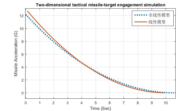Fig. 2.7 Linearized engagement model yields accurate performance projections for heading error disturbance. 图 2.7 线性交战模型可以精准预测航向误差干扰下的导弹特性

To verify that the linearized engagement model is a reasonable approximation to the nonlinear engagement model, cases that were run for the nonlinear engagement model were repeated using the simulation of Listing 2.2. A sample run was made with the linearized engagement model in which the only disturbance was a -20deg heading error ( HEDEG = –20. ). In this case the effective navigation ratio was 4. Acceleration profile comparisons for both the linear and nonlinear engagement models are presented in Fig. 2.7. The figure clearly shows that, even for a relatively large heading error disturbance, the resultant acceleration profiles are virtually indistinguishable. Thus, the linearized model is an excellent approximation to the nonlinear engagement model in the case of a heading error disturbance.

为了验证线性交战模型能否实现对非线性交战模型的合理近似，再次使用表2.2中的代码对非线性交战模型进行仿真。以-20度航向误差（HEDEG= –20）作为唯一的干扰，对线性化交战模型进行了一次仿真，其中有效导航比为4。所得线性和非线性交战模型的加速度包络对比图如图2.7所示。从图中可以清楚地看出，即使在相对较大的航向误差扰动下，所得到的两条加速度包络曲线也几乎无法区分。因此，在对航向误差扰动情况进行仿真时，线性化模型可以很好的实现对非线性交战模型的近似。

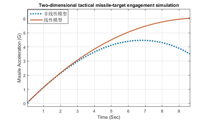
Fig. 2.8 Linear model overestimates missile acceleration due to target maneuver.
图 2.8 线性模型高估了由目标机动引发的导弹加速度大小
Another sample run was made with the linear engagement model; this time with a 3-g target maneuver disturbance. Figure 2.8 shows that this time the linearized model overestimates the missile acceleration requirements. The reason for the discrepancy is that the linear model assumes that the target acceleration magnitude, perpendicular to the line of sight, is always the same and equal to the magnitude of the maneuver. In reality, as the target maneuvers, the component of acceleration perpendicular to the line of sight decreases because the target is turning. Therefore, the nonlinear acceleration requirements due to a maneuvering target are somewhat less than those predicted by the linearized engagement model. However, it is important to note that the linear engagement model accurately predicts the monotonically increasing trend (for most of the flight) for the missile acceleration profile due to a target maneuver.

同理，使用线性交战模型，对3g目标机动干扰条件进行仿真。图2.8显示，线性化模型高估了导弹对加速度的需求。产生差异的原因是，线性模型假设目标加速度始终垂直于弹目视线，且的加速度大小是不变的。而实际上，当目标机动时目标速度不断发生偏转，垂直于弹目视线的加速度分量会不断减小。因此非线性模型中，导弹为应对目标机动所需的加速度大小略小于线性交战模型给出的结果。尽管如此，（在大多数飞行条件下）线性交战模型依然可以准确预测由目标机动引发的导弹加速度包络的单调递增趋势。

At this point we can conclude that the linearized engagement model yields performance projections of sufficient accuracy to make it worthwhile to proceed with the development of design relationships. We will test the validity of those relationships throughout the text in a variety of environments.
在这一点上，我们可以得出结论，线性交战模型可对导弹性能进行足够精确的预测，值得我们在“弹目相对运动关系”的设计开发中继续关注。在本书将在各种环境中测试线性模型的有效性。

IMPORTANT CLOSED-FORM SOLUTIONS 重要的解析解

译者注：此处的 closed-form solutions 应直译为闭式解、封闭解，有说法表示也可等效为解析解(analytical solution)。译者认为作者在本文所提到的closed-form solutions应该是相对于numerical solution（数值解）而言，而不用过度纠结闭式解与解析解之间的差异，因此为了便于理解，本文中统一将 closed-form solutions 翻译为解析解，泛指通过数学公式推导所得到的解的表达式。

The linearization of the engagement model is important for two reasons. First, with a linear model, powerful computerized techniques such as the method of adjoints (described in Chapters 3 and 4) can be used to analyze the missile guidance system both statistically and deterministically in one computer run. With this technique, error budgets are automatically generated so that key system drivers can be identified and a balanced guidance system design can be achieved. The linear model is also important because, under special circumstances, closed-form solutions can be obtained. These solutions can be used as system sizing aids. In addition, the form of the solutions will suggest how key parameters influence system performance.
交战模型的线性化工作非常重要，主要出于两个原因。首先，基于线性模型，一些强大的“数学工具”（如第3章和第4章所述的伴随法）可用于导弹制导系统的分析，通过一次仿真运算就可同时完成统计性和确定性分析。利用该技术 （此处指伴随法） ，可得到系统对不同误差的容忍度，进而识别出影响系统特性的关键因素，从而实现均衡的制导系统设计。另一个重要的原因是，在特殊情况下，可以通过线性模型获得微分方程组的解析解。这些解析解可用作系统评估的工具，且通过解析解的形式可反应出各关键系数对系统性能的影响。

译者注：system sizing这里翻译为系统评估

Let us consider obtaining closed-form solutions for the two important cases we have already considered in both the linear and nonlinear engagement simulations. The first case is the missile acceleration required to remove a heading error, and the second case is the missile acceleration required to hit a maneuvering target. In the absence of target maneuver the relative acceleration (target acceleration minus missile acceleration) can be expressed as

以上文提到的线性和非线性交战仿真中的两个重要场景为例，尝试求取其解析解。场景一是求取为消除航向误差所需产生的导弹加速度，场景二是求取为命中机动目标所需产生的导弹加速度。在不考虑目标机

动的情况下，相对加速度（目标加速度减去导弹加速度）可以表示为

$$\ddot{y}=-N^{\prime }{V}_c\dot{\lambda }$$

Integrating the preceding differential equation once yields
将上述微分方程进行一次积分得

$$\dot{y}=-N^{\prime }{V}_c\lambda +C_1$$

where $C_1$ is the constant of integration. Substitution of the linear approximation to the line-of-sight angle in the preceding expression yields the following time-varying first-order differential equation:
其中$C_1$是积分常数。将视线角的线性近似值代入上式，得到以下一阶时变微分方程：

$$\frac{dy}{dt}+\frac{N^{\prime }y}{t_F-t}=C_1$$

As a first-order differential equation of the form
作为形如下式的一阶微分方程

$$\frac{dy}{dt}+a(t)y=h(t)$$

has the solution [9–12]
具有如下形式的解
$$y=exp[-{\int }_0^{t}a(T)dT]\{{\int }_0^{t}h(n)exp[{\int }_0^{n}a(T)dT]dn+C_2\}$$

we can solve the linearized trajectory differential equation exactly. Note that the first constant of integration $C_1$ is contained in $h(t)$ while the second constant of integration $C_2$ appears in the preceding equation. Both constants of integration can be found by evaluating initial conditions on y and its derivative. Let us assume that the initial condition on the first state is zero, or
利用上式，我们可以精确地求解线性化的轨迹微分方程。注意，第一个积分常数$C_1$包含在$h(t)$中，而第二个积分常数$C_2$出现在前面的等式中。这两个积分常数都可以通过计算$y$及其导数的初始条件来获得。让我们假设第一个状态量的初始条件为零，或者

$$y(0)=0$$

and that the initial condition on the second state is related to the heading error by
第二个状态量的初始条件与航向误差相关

$$\dot{y}(0)=-V_{M}HE$$

where $V_M$ is the missile velocity and $HE$ the heading error in radians. Under these circumstances, after much algebra, we find that the closed-form solution for the missile acceleration due to heading error is given by
其中$V_M$是导弹速度，$HE$是以弧度表示的航向误差。在这种情况下，经过大量代数运算，我们可得到由航向误差所致导弹加速度的解析解如下所示

$$n_c=\frac{-V_{M}HE{N}^{\prime }}{t_F}(1-\frac{t}{t_F}{)}^{N^{\prime }-2}$$

where $t_F$ is the flight time and $N^{\prime }$ the effective navigation ratio. We can see that the magnitude of the initial acceleration is proportional to the heading error and missile velocity and inversely proportional to the flight time. Doubling the velocity or heading error will double the initial missile acceleration, whereas doubling the flight time or time available for guidance will halve the initial missile acceleration. In addition, the closed-form solution for the miss distance $y(t_F)$ is zero. In other words, as long as the missile has sufficient acceleration capability, there is no miss due to heading error!
其中$t_F$是总飞行时间，$N^{\prime }$是有效导引比。我们可以看到，初始加速度的大小与航向误差以及导弹速度成正比，与总飞行时间成反比。如果速度或航向误差增加一倍将使导弹初始加速度需求增加一倍，而如果飞行时间（即，可用于制导的时间）增加一倍则将使导弹的初始加速度需求减少一半。此外，脱靶量$y_{(}tF)$的解析解为零。换言之，只要导弹有足够的加速能力，就不会因为航向误差的存在而脱靶！

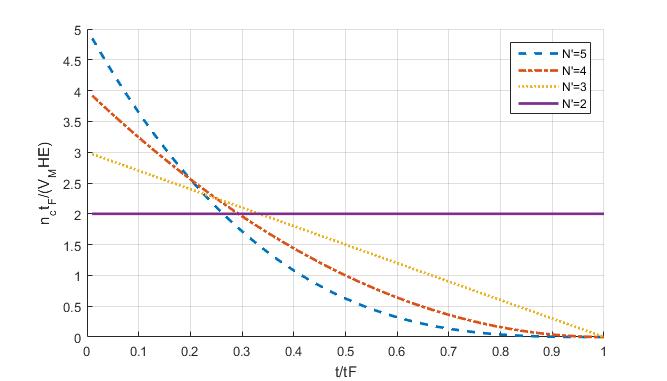
Fig. 2.9 Normalized missile acceleration due to heading error for proportional navigation guidance.
图2.9 比例导引律下航向误差所致归一化导弹加速度

The closed-form solution for the missile acceleration response due to heading error is displayed in normalized form in Fig. 2.9. We can see that higher effective navigation ratios require more acceleration at the beginning of flight than at the end of the flight and less acceleration as the flight progresses. From a system sizing point of view, the designer usually wants to ensure that the acceleration capability of the missile is adequate at the beginning of flight so that saturation can be avoided. For a fixed missile acceleration capability, Fig. 2.9 shows how requirements are placed on minimum guidance or flight time and maximum allowable heading error and missile velocity.

由航向误差所致导弹加速度响应的解析解以归一化的形式显示在图2.9中。我们可以看到，增大有效导引比会增大制导段始、末导弹对加速度需求的差异，且随着弹道推进导弹对加速度的需求逐步减少。从系统评估的角度来看，设计师们通常会确保导弹在制导初段时具有足够的加速能力，从而避免 (全制导过程中出现加速度) 饱和现象的产生。图2.9显示了，在一定的导弹加速能力下，最小制导时间(或总飞行时间)、最大允许航向误差和导弹速度之间的制衡关系。

Similarly, if the only disturbance is a target maneuver, the appropriate second-order differential equation becomes
类似地，如果将目标机动设定为唯一的干扰，则的二阶微分方程变为

$$\ddot{y}=-N^{\prime }{V}_c\dot{\lambda }+n_T$$

with initial conditions
在如下初始条件下

$$y(0)=0$$
$$\dot{y}(0)=0$$

After conversion to a first-order differential equation and much algebra, the solution can be found to be
转换成一阶微分方程，并经过若干代数运算之后，可以得到解为

$$n_c=\frac{N^{\prime }}{N^{\prime }-2}[1-(1-\frac{t}{t_F}{)}^{N^{\prime }-2}]n_T$$

It appears that something “magical” happens to the acceleration when the effective navigation ratio is two. Application of L‘Hopital’s rule eliminates the division by zero in the preceding formula and indicates that

当有效导引比为2时，加速度似乎发生了“神奇”的变化。使用L‘Hopital法则，消除了上式中的分母为0项，并得到
$$\underset{n\to +\infty }{\lim }{n}_c=-2ln\left(\frac{t_F-t}{t_F}\right)$$

This is approximately the same solution as if we simply let N’ = 2.01 or N’ = 1.99 in the original closed-form solution for the acceleration as a function of the effective navigation ratio. As with the heading error case, the closed-form solution indicates that the miss distance due to target maneuver is exactly zero!

（如果不想使用L‘Hopital法则，解决分母为零的问题） 我们也可以将原本$n_c$的解析解表达式看做有效导引比N’的函数，并直接将N’ = 2.01或N’ = 1.99带入其中。与航向误差的场景相同，解析解表明目标机动场景中脱靶量也正好为零！

Unlike the heading error case, missile acceleration due to maneuver is independent of flight time and missile velocity and only depends on the magnitude of the maneuver and the effective navigation ratio. Doubling the maneuver level of the target doubles the missile acceleration requirements.
与航向误差场景不同的是，目标机动所致导弹加速度与制导时间和导弹速度无关，仅取决于机动幅度和有效导引比。若将目标的机动水平提高一倍，则导弹的加速需求就提高一倍。

Fig. 2.10 Normalized missile acceleration due to target maneuver for proportional navigation guidance.
图2.10 比例导引律所得归一化后由目标机动所致导弹加速度曲线

The closed-form solution for the missile acceleration response due to target maneuver is displayed in normalized form in Fig. 2.10. We can see that higher effective navigation ratios relax the acceleration requirements at the end of the flight. Unlike the heading error response, the missile acceleration required to hit a maneuvering target increases as the flight progresses. From a system sizing point of view, the designer must ensure that the acceleration capability of the missile is adequate at the end of flight so that saturation can be avoided so that the missile can hit the target.
图2.10以归一化的形式显示了目标机动所致导弹加速度响应的解析解。可见，选择更高的有效导引比可降低飞行结束时导弹的加速度需求。与航向误差场景的响应不同，为命中机动目标所需的导弹加速度随着弹道的推进而增加。从系统评估的角度来看，设计师必须确保导弹在飞行结束时具有足够的机动能力，避免加速度饱和现象的产生，进而保证导弹能够命中目标。

PROPORTIONAL NAVIGATION AND ZERO EFFORT MISS 比例导航与零脱靶量

Thus far we have seen from simulation results and closed-form solutions that proportional navigation appears to be effective, but we do not know why. Although it is possible to construct geometric arguments showing that it is very logical to issue acceleration commands proportional to the line-of-sight rate (that is, zero line-of-sight rate means we are on a collision triangle and therefore no further commands are necessary), it is not obvious what is happening. The concept of zero effort miss is not only useful in explaining proportional navigation but is also useful in deriving and understanding more advanced guidance laws.

到目前为止，我们似乎已经可以从仿真结果和解析解中体会到比例导引律的有效性，但却不清楚其有效的原因。虽然可以从几何构型上来说明加速度指令与视线速度成比例是非常合乎逻辑的（即，视线速度为零意味着导弹和目标处于碰撞三角形上，因此加速度指令也为0），但却不能直观的解释比例导引的过程中究竟发生了什么 (才能保证零脱靶量的效果)。为了进一步解释比例导引的作用，需要引入零作用力脱靶量的概念，这个概念在推导和理解更先进的制导律时也起到了重要的作用。

译者注：比例导引的原理非常简单而合理，如果导弹和目标均保持当前状态飞行就可以命中目标，则在导弹抵近目标过程中，弹目连线只会平移，而不会旋转，即弹目连线与地理系的夹角保持不变，视线角速率为零，因而根据比例导引律，产生的加速度为0。而如果随着目标的抵近弹目视线角发生了变化，说明由于误差的存在，弹目并未处于碰撞三角形中，根据比例导引律产生一个与视线角速度成比例的加速度以改变导弹航向，使得导弹与目标重新回到碰撞三角形中。因此比例导引的目的是通过导弹产生加速度使得视线角速度变为0.

译者注：比例导引类似P控制，理论上会存在静差，即由于观测误差的存在，当过载为0时角速率可能会存在一个残差小值，也就是说导弹和目标没有完美的处于碰撞三角形中，理论上一定存在一些脱靶量。但好在脱靶量与视线角速度之间并非比例关系，随着弹目距离的减小，脱靶量引起的视线角速率会逐步增大，从而进一步产生导弹加速度以缩小脱靶量。

We can define the zero effort miss to be the distance the missile would miss the target if the target continued along its present course and the missile made no further corrective maneuvers. Therefore, if the target does not maneuver, the two components, in the Earth fixed coordinate system, of the zero effort miss can be expressed in terms of the previously defined relative quantities as
我们将零作用力脱靶量定义为，目标继续沿着当前航线飞行且导弹不再进一步进行机动修正时的脱靶量。因此，如果目标不执行机动动作，则在地球坐标系中零作用力脱靶量的两个分量可以用上文定义的相对量表示为

$$ZE{M}_1=R_{TM1}+V_{TM1}{t}_{go}$$
$$ZE{M}_2=R_{TM2}+V_{TM2}{t}_{go}$$

where $t_{go}$ is the time to go until intercept. Thus, we can see that in this case the zero effort miss is just a simple prediction (assuming constant velocities and zero acceleration) of the future relative separation between missile and target. From Fig. 2.1 we can see that the component of the zero effort miss that is perpendicular to the line of sight $ZE{M}_{PLOS}$ can be found by trigonometry and is given by
其中$t_{go}$是命中前的剩余制导时间。由此可见，在这种情况下零作用力脱靶量只是对导弹和目标间相对距离的简单预测（假设恒定速度和零加速度）。如图2.1所示，可利用几何三角关系得到垂直于视线的零作用力脱靶量的分量$ZE{M}_{PLOS}$，表示为

$$ZE{M}_{PLOS}=-ZE{M}_{1}sin\lambda +ZE{M}_{2}cos\lambda$$

Expansion and simplification of the preceding equation yields
展开并简化上式得到

$$ZE{M}_{PLOS}=\frac{t_{go}(R_{TM1}{V}_{TM2}-R_{TM2}{V}_{TM1})}{R_{TM}}$$

Comparing the preceding expression to the expression for line-of-sight rate, we can see that the line-of-sight rate can be expressed in terms of the component of the zero effort miss perpendicular to the line of sight or
将上式与视线速率的表达式进行比较，我们可以看到视线速率可以用垂直于视线的零作用脱靶量分量来表示，即

$$\dot{\lambda }=\frac{ZE{M}_{PLOS}}{R_{TM}{t}_{go}}$$

If we assume that the relative separation between missile and target and closing velocity are approximately related to the time to go by
如果我们假设导弹和目标之间的相对距离和接近速度大致与飞行时间有如下关系

$$R_{TM}=V_c{t}_{go}$$

then the proportional navigation guidance command can be expressed in terms of the zero effort miss perpendicular to the line sight as
那么比例导引产生的制导命令可以用垂直于视线的零作用力脱靶量表示为

$$n_c=\frac{N^{\prime }ZE{M}_{PLOS}}{t_{go}^2}$$

Thus, we can see that the proportional navigation acceleration command that is perpendicular to the line of sight is not only proportional to the line-of-sight rate and closing velocity but is also proportional to the zero effort miss and inversely proportional to the square of time to go. We shall see later (in Chapters 8, 15, and 20) that this is a very powerful concept, as the zero effort miss can be computed by a variety of methods, including the on-line numerical integration of the assumed nonlinear differential equations of the missile and target.
因此我们可以看到，比例导引律所产生垂直于视线的加速度指令不仅与视线角速度和抵近速度成正比，而且与零作用力脱靶量成正比，与剩余飞行时间平方成反比。我们稍后（在第8、15和20章）将会看到，上式是一个非常好用的概念，因为我们可以利用多种方法计算得到零作用力脱靶量，包括对弹目非线性微分方程进行在线数值积分。

SUMMARY 总结

In this chapter we have developed and shown the results of a simple two dimensional proportional navigation missile-target engagement simulation. Results have shown that the proportional navigation law is effective in a variety of cases. Linearization of the nonlinear missile-target geometry was shown to be an accurate approximation to the actual geometry. Closed-form solutions were derived, based on the linearized geometry, for the missile acceleration requirements due to heading error and target maneuver. From these solutions it was shown how the effective navigation ratio influences system performance. Finally, the concept of zero effort miss was introduced, and it was shown how the proportional navigation guidance law could be expressed in terms of this concept. Later (Chapters 8, 15, and 20), we shall develop more advanced guidance laws based upon the zero effort miss concept.
在本章中，我们给出并编程实现了一个简易二维比例导引弹目交战模型的仿真结果。结果表明，比例导引法可以有效应对多种交战情况。证明了对非线性弹目几何关系的线性化结果可实现对真实几何关系的精确近似。基于线性化几何关系，推导出了由航向误差和目标机动所致导弹加速度需求的解析解。通过这些解析解可以说明有效导引比是如何影响系统性能的。最后，引入了零作用力脱靶量的概念，并展示了如何根据该概念表示比例导引律。稍后（第8章、第15章和第20章），我们将基于零作用力脱靶量的概念提出更先进的制导法则。

REFERENCES 参考文献

[1] Kennedy, G. P., Rockets, Missiles and Spacecraft of the National Air and Space
Museum, Smithsonian Institution Press, Washington, DC, 1983.
[2] Benecke, T., and Quick, A. W. (eds.), “History of German Guided Missile
Development,” Proceedings of AGARD First Guided Missile Seminar, 1956.
[3] Nesline, F. W., and Zarchan, P., “A New Look at Classical Versus Modern Homing
Guidance,” Journal of Guidance and Control, Vol. 4, Jan.–Feb. 1981, pp. 78–85.
[4] Yuan, C. L., “Homing and Navigation Courses of Automatic Target-Seeking Devices,”
RCA Labs., Rept. PTR-12C, Princeton, NJ, Dec. 1942.
[5] Bennett, R. R., and Mathews, W. E., “Analytical Determination of Miss Distance for
Linear Homing Navigation Systems,” Hughes Aircraft Co., TN-260, Culver City, CA,
March 1952.
[6] Fossier, M. W., “The Development of Radar Homing Missiles,” Journal of Guidance,
Control, and Dynamics, Vol. 7, Nov.–Dec. 1984, pp. 641–651.
[7] Yuan, C. L., “Homing and Navigation Courses of Automatic Target-Seeking Devices,”
Journal of Applied Physics, Vol. 19, Dec. 1948, pp. 1122–1128.
[8] Bryson, A. E., and Ho, Y. C., Applied Optimal Control, Blaisdell, Waltham, MA, 1969.