pandas-task10-时序数据.md

最新推荐文章于 2023-12-07 16:22:09 发布

Alex好好干饭

最新推荐文章于 2023-12-07 16:22:09 发布

阅读量337

点赞数 1

分类专栏： pandas 文章标签： pandas 深度学习数据挖掘

本文链接：https://blog.csdn.net/weixin_37734833/article/details/112350770

版权

pandas 专栏收录该内容

12 篇文章 0 订阅

订阅专栏

文章目录

一、时序中的基本对象
二、时间戳
三、时间差
- 1. Timedelta的生成
- 2. Timedelta的运算
四、日期偏置
- 1. Offset对象
- 2. 偏置字符串
五、时序中的滑窗与分组
- 1. 滑动窗口
- 2. 重采样
六、练习
- Ex1：太阳辐射数据集
- Ex2：水果销量数据集

本周末期末考试三门需要复习只能大概快速梳理一下了写了下练习题写的不全请见谅之后会补上

一、时序中的基本对象

时间序列的概念在日常生活中十分常见，但对于一个具体的时序事件而言，可以从多个时间对象的角度来描述。例如2020年9月7日周一早上8点整需要到教室上课，这个课会在当天早上10点结束，其中包含了哪些时间概念？

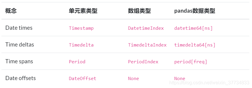
第一，会出现时间戳（Date times）的概念，即’2020-9-7 08:00:00’和’2020-9-7 10:00:00’这两个时间点分别代表了上课和下课的时刻，在 pandas 中称为 Timestamp 。同时，一系列的时间戳可以组成 DatetimeIndex ，而将它放到 Series 中后， Series 的类型就变为了 datetime64[ns] ，如果有涉及时区则为 datetime64[ns, tz] ，其中tz是timezone的简写。
第二，会出现时间差（Time deltas）的概念，即上课需要的时间，两个 Timestamp 做差就得到了时间差，pandas中利用 Timedelta 来表示。类似的，一系列的时间差就组成了 TimedeltaIndex ，而将它放到 Series 中后， Series 的类型就变为了 timedelta64[ns] 。
第三，会出现时间段（Time spans）的概念，即在8点到10点这个区间都会持续地在上课，在 pandas 利用 Period 来表示。类似的，一系列的时间段就组成了 PeriodIndex ，而将它放到 Series 中后， Series 的类型就变为了 Period 。
第四，会出现日期偏置（Date offsets）的概念，假设你只知道9月的第一个周一早上8点要去上课，但不知道具体的日期，那么就需要一个类型来处理此类需求。再例如，想要知道2020年9月7日后的第30个工作日是哪一天，那么时间差就解决不了你的问题，从而 pandas 中的 DateOffset 就出现了。同时， pandas 中没有为一列时间偏置专门设计存储类型，理由也很简单，因为需求比较奇怪，一般来说我们只需要对一批时间特征做一个统一的特殊日期偏置。

通过这个简单的例子，就能够容易地总结出官方文档中的这个表格：
在这里插入图片描述
由于时间段对象 Period/PeriodIndex 的使用频率并不高，因此将不进行讲解，而只涉及时间戳序列、时间差序列和日期偏置的相关内容。

二、时间戳

1. Timestamp的构造与属性

单个时间戳的生成利用 pd.Timestamp 实现，一般而言的常见日期格式都能被成功地转换。

通过 year, month, day, hour, min, second 可以获取具体的数值。

在 pandas 中，时间戳的最小精度为纳秒 ns ，由于使用了64位存储，可以表示的时间范围大约可以如下计算：
$\rm Time\,Range = \frac{2^{64}}{10^9\times 60\times 60\times 24\times 365} \approx 585 (Years)$
通过 pd.Timestamp.max 和 pd.Timestamp.min 可以获取时间戳表示的范围。

2. Datetime序列的生成

一组时间戳可以组成时间序列，可以用 to_datetime 和 date_range 来生成。其中， to_datetime 能够把一列时间戳格式的对象转换成为 datetime64[ns] 类型的时间序列

3. dt对象

如同 category, string 的序列上定义了 cat, str 来完成分类数据和文本数据的操作，在时序类型的序列上定义了 dt 对象来完成许多时间序列的相关操作。这里对于 datetime64[ns] 类型而言，可以大致分为三类操作：取出时间相关的属性、判断时间戳是否满足条件、取整操作。

第一类操作的常用属性包括： date, time, year, month, day, hour, minute, second, microsecond, nanosecond, dayofweek, dayofyear, weekofyear, daysinmonth, quarter ，其中 daysinmonth, quarter 分别表示月中的第几天和季度。

4. 时间戳的切片与索引

一般而言，时间戳序列作为索引使用。如果想要选出某个子时间戳序列，第一类方法是利用 dt 对象和布尔条件联合使用，另一种方式是利用切片，后者常用于连续时间戳。

三、时间差

1. Timedelta的生成

正如在第一节中所说，时间差可以理解为两个时间戳的差，这里也可以通过 pd.Timedelta 来构造。

2. Timedelta的运算

四、日期偏置

1. Offset对象

2. 偏置字符串

五、时序中的滑窗与分组

1. 滑动窗口

所谓时序的滑窗函数，即把滑动窗口用 freq 关键词代替，下面给出一个具体的应用案例：在股票市场中有一个指标为 BOLL 指标，它由中轨线、上轨线、下轨线这三根线构成，具体的计算方法分别是 N 日均值线、 N 日均值加两倍 N 日标准差线、 N 日均值减两倍 N 日标准差线。

2. 重采样

重采样对象 resample 和第四章中分组对象 groupby 的用法类似，前者是针对时间序列的分组计算而设计的分组对象。

六、练习

Ex1：太阳辐射数据集

现有一份关于太阳辐射的数据集：
在这里插入图片描述

将 Datetime, Time 合并为一个时间列 Datetime ，同时把它作为索引后排序。

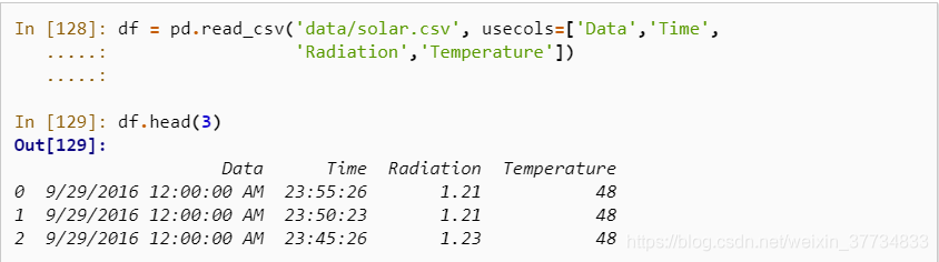
先看下表格什么样子：

df = pd.read_csv('data/solar.csv', usecols=['Data','Time',
                     'Radiation','Temperature'])
df.head(3)

	Data	Time	Radiation	Temperature
0	9/29/2016 12:00:00 AM	23:55:26	1.21	48
1	9/29/2016 12:00:00 AM	23:50:23	1.21	48
2	9/29/2016 12:00:00 AM	23:45:26	1.23	48

利用正则表达式获取日期，将日期和时间合并成时间列。
这里正则表达式我没有和答案完全一样，答案给的是 ‘([/|\w]+\s).+’)，个人觉得后面的.+好像没有必要，试了下对结果也没影响。

day_of_year=df.Data.str.extract(r'([/|\w]+)')[0]
df['Datetime']=pd.to_datetime(day_of_year +' '+ df.Time)
df.head(3)

	Data	Time	Radiation	Temperature	Datetime
0	9/29/2016 12:00:00 AM	23:55:26	1.21	48	2016-09-29 23:55:26
1	9/29/2016 12:00:00 AM	23:50:23	1.21	48	2016-09-29 23:50:23
2	9/29/2016 12:00:00 AM	23:45:26	1.23	48	2016-09-29 23:45:26

然后再设置index及排序即可：

df.set_index('Datetime').sort_index(ascending=True).head(5)

	Data	Time	Radiation	Temperature	Datetime
0	9/29/2016 12:00:00 AM	23:55:26	1.21	48	2016-09-29 23:55:26
1	9/29/2016 12:00:00 AM	23:50:23	1.21	48	2016-09-29 23:50:23
2	9/29/2016 12:00:00 AM	23:45:26	1.23	48	2016-09-29 23:45:26
3	9/29/2016 12:00:00 AM	23:40:21	1.21	48	2016-09-29 23:40:21
4	9/29/2016 12:00:00 AM	23:35:24	1.17	48	2016-09-29 23:35:24

这里忘记把原来的两列Data和Time删除了，使用drop删除：

df=df.drop(columns=['Data','Time']).
        set_index('Datetime').sort_index(ascending=True)

Datetime	Radiation	Temperature
2016-09-01 00:00:08	2.58	51
2016-09-01 00:05:10	2.83	51
2016-09-01 00:20:06	2.16	51
2016-09-01 00:25:05	2.21	51
2016-09-01 00:30:09	2.25	51

每条记录时间的间隔显然并不一致，请解决如下问题：
a. 找出间隔时间的前三个最大值所对应的三组时间戳。

s = df.index.to_series().reset_index(drop=True).diff().dt.total_seconds()
max_3 = s.nlargest(3).index
df.index[max_3.union(max_3-1)]
# DatetimeIndex(['2016-09-29 23:55:26', '2016-10-01 00:00:19',
#                '2016-11-29 19:05:02', '2016-12-01 00:00:02',
#                '2016-12-05 20:45:53', '2016-12-08 11:10:42'],
#               dtype='datetime64[ns]', name='Datetime', freq=None)

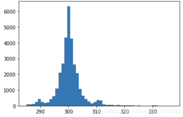
b. 是否存在一个大致的范围，使得绝大多数的间隔时间都落在这个区间中？如果存在，请对此范围内的样本间隔秒数画出柱状图，设置 bins=50 。

import matplotlib.pyplot as plt
res = s.mask((s>s.quantile(0.99))|(s<s.quantile(0.01)))
_ = plt.hist(res, bins=50)

在这里插入图片描述
3. 求如下指标对应的 Series ：
a. 温度与辐射量的6小时滑动相关系数

res = df.Radiation.rolling('6H').corr(df.Temperature)
res.tail(3)
# Datetime
# 2016-12-31 23:45:04    0.328574
# 2016-12-31 23:50:03    0.261883
# 2016-12-31 23:55:01    0.262406
# dtype: float64

b.以三点、九点、十五点、二十一点为分割，该观测所在时间区间的温度均值序列

res = df.Temperature.resample('6H', origin='03:00:00').mean()
res.head()
# Datetime
# 2016-08-31 21:00:00    51.218750
# 2016-09-01 03:00:00    50.033333
# 2016-09-01 09:00:00    59.379310
# 2016-09-01 15:00:00    57.984375
# 2016-09-01 21:00:00    51.393939
# Freq: 6H, Name: Temperature, dtype: float64

c.每个观测6小时前的辐射量（一般而言不会恰好取到，此时取最近时间戳对应的辐射量）

my_dt = df.index.shift(freq='-6H')

int_loc = [df.index.get_loc(i, method='nearest') for i in my_dt]

res = df.Radiation.iloc[int_loc]

res.tail(3)
# Datetime
# 2016-12-31 17:45:02    9.33
# 2016-12-31 17:50:01    8.49
# 2016-12-31 17:55:02    5.84
# Name: Radiation, dtype: float64

Ex2：水果销量数据集

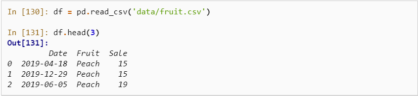
现有一份2019年每日水果销量记录表：
在这里插入图片描述

统计如下指标：
a. 每月上半月（15号及之前）与下半月葡萄销量的比值

df = pd.read_csv('data/fruit.csv')
df.Date = pd.to_datetime(df.Date)
df_grape = df.query("Fruit == 'Grape'")
res = df_grape.groupby([np.where(df_grape.Date.dt.day<=15,
                            'First', 'Second'),df_grape.Date.dt.month]
                            )['Sale'].mean().to_frame().unstack(0
                            ).droplevel(0,axis=1)
res = (res.First/res.Second).rename_axis('Month')
res.head()
# Month
# 1    1.174998
# 2    0.968890
# 3    0.951351
# 4    1.020797
# 5    0.931061
# dtype: float64

b.每月最后一天的生梨销量总和

df[df.Date.dt.is_month_end].query("Fruit == 'Pear'"
                              ).groupby('Date').Sale.sum().head()
# Date
# 2019-01-31    847
# 2019-02-28    774
# 2019-03-31    761
# 2019-04-30    648
# 2019-05-31    616
# Name: Sale, dtype: int64

c.每月最后一天工作日的生梨销量总和

df[df.Date.isin(pd.date_range('20190101', '20191231',
                    freq='BM'))].query("Fruit == 'Pear'"
                    ).groupby('Date').Sale.mean().head()
# Date
# 2019-01-31    60.500000
# 2019-02-28    59.538462
# 2019-03-29    56.666667
# 2019-04-30    64.800000
# 2019-05-31    61.600000
# Name: Sale, dtype: float64

d.每月最后五天的苹果销量均值

target_dt = df.drop_duplicates().groupby(df.Date.drop_duplicates(
                ).dt.month)['Date'].nlargest(5).reset_index(drop=True)

res = df.set_index('Date').loc[target_dt].reset_index(
                ).query("Fruit == 'Apple'")

res = res.groupby(res.Date.dt.month)['Sale'].mean(
                ).rename_axis('Month')

res.head()
# Month
# 1    65.313725
# 2    54.061538
# 3    59.325581
# 4    65.795455
# 5    57.465116
# Name: Sale, dtype: float64

按月计算周一至周日各品种水果的平均记录条数，行索引外层为水果名称，内层为月份，列索引为星期。

month_order = ['January','February','March','April',
                    'May','June','July','August','September',
                    'October','November','December']
    

week_order = ['Mon','Tue','Wed','Thu','Fri','Sat','Sum']

group1 = df.Date.dt.month_name().astype('category').cat.reorder_categories(
            month_order, ordered=True)

group2 = df.Fruit

group3 = df.Date.dt.dayofweek.replace(dict(zip(range(7),week_order))
             ).astype('category').cat.reorder_categories(
             week_order, ordered=True)

res = df.groupby([group1, group2,group3])['Sale'].count().to_frame(
             ).unstack(0).droplevel(0,axis=1)

res.head()

在这里插入图片描述

按天计算向前10个工作日窗口的苹果销量均值序列，非工作日的值用上一个工作日的结果填

df_apple = df[(df.Fruit=='Apple')&(
                  ~df.Date.dt.dayofweek.isin([5,6]))]

s = pd.Series(df_apple.Sale.values,
                  index=df_apple.Date).groupby('Date').sum()

res = s.rolling('10D').mean().reindex(
                  pd.date_range('20190101','20191231')).fillna(method='ffill')

res.head()
# 2019-01-01    189.000000
# 2019-01-02    335.500000
# 2019-01-03    520.333333
# 2019-01-04    527.750000
# 2019-01-05    527.750000
# Freq: D, dtype: float64

Alex好好干饭

关注

1
点赞
踩
1

收藏

觉得还不错? 一键收藏
1
评论
pandas-task10-时序数据.md

文章目录一、时序中的基本对象二、时间戳三、时间差四、日期偏置五、时序中的滑窗与分组六、练习Ex1：太阳辐射数据集Ex2：水果销量数据集本周末期末考试三门需要复习只能大概快速梳理一下了写了下练习题写的不全请见谅之后会补上一、时序中的基本对象二、时间戳三、时间差四、日期偏置五、时序中的滑窗与分组六、练习Ex1：太阳辐射数据集现有一份关于太阳辐射的数据集：将 Datetime, Time 合并为一个时间列 Datetime ，同时把它作为索引后排序。先看下表格什么样子：d
复制链接

扫一扫