


1、环境
python: 3.8
pytorch: 1.7
cudnn: 安一个对应你电脑的版本就可以
2、NTU RGB+D数据集下载
由于下载NTU-RGB+D数据集特别的慢,这里博主就使用的别人下载好并划分出来的数据集进行训练和验证的,其次本文复现并没有使用kinetics数据集,因为博主由于课题原因只需要使用到三维的骨骼关节点数据,因此并没有对kinetics数据集的结果进行复现。
由于百度网盘无法上传整个项目,这里给出paddle上面给出的数据集下载地址,应该比outer要快不少,或者自己去paddle paddle找一下数据集:
首先去github下载源码:https://github.com/yysijie/st-gcn
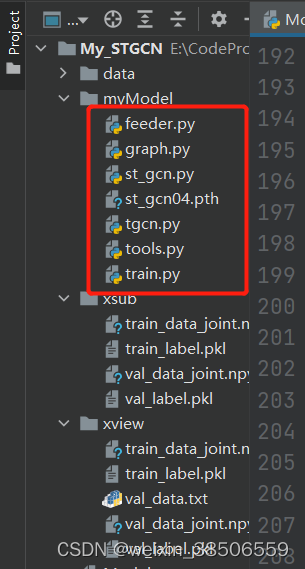
下载源码后,我们主要看这三个文件夹:

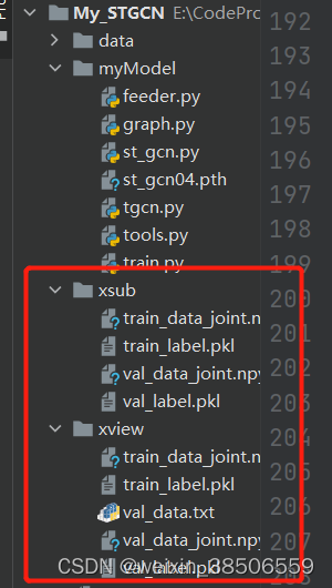
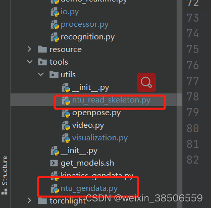
我们可以将这几个文件夹里面的feeder.py, st_gcn.py, tgcn.py,以及tools.py文件拿出来,自己建一个新的项目:一个是项目文件,一个是两个数据集x-sub和x-view,都是下载的别人处理后。如果是没处理的数据的话,再把另个相关与ntu处理相关的.py文件也拿过来运行后即可生成对应的.pkl和.npy文件。
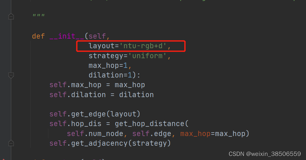
这里还需要修改一下graph.py文件这一行:
下面自己创建一个train.py文件,由于源码中的训练代码配置了很多的参数,写了太多,看的时候感觉不是很清晰,就自己找了一个类似的训练脚本跟着修改的:
这里由于我在自己的电脑上跑的,电脑性能不是很好,所以batch_size设为8,其实出来的效果不是很理想。可以试试多gpu增大batch_size试试,我看源码的demo设置的是4个gpu, batch_size=64。
import torch
import numpy as np
from myModel.feeder import Feeder
from st_gcn import Model
NUM_EPOCH = 100
BATCH_SIZE = 8

# 模型
model = Model(num_class=60, in_channels=3, dropout=0.5).cuda()

# 优化器
# optimizer = torch.optim.SGD(model.parameters(), lr=0.01, momentum=0.9)
optimizer = torch.optim.RMSprop(model.parameters(), lr=0.001)

# 误差函数
criterion = torch.nn.CrossEntropyLoss()

# 加载数据
data_loader = dict()
data_loader['train'] = torch.utils.data.DataLoader(
    dataset=Feeder(data_path='../xview/train_data_joint.npy',
                   label_path='../xview/val_label.pkl'),
    batch_size=BATCH_SIZE, shuffle=True, num_workers=0)
data_loader['test'] = torch.utils.data.DataLoader(
    dataset=Feeder(data_path='../xview/val_data_joint.npy',
                   label_path='../xview/val_label.pkl'),
    batch_size=BATCH_SIZE, shuffle=False, num_workers=0)

# 模型训练
print("------------------Training-------------------------")
model.train()
best_acc = 0.0
save_path = './st_gcn04.pth'
val_num = len(data_loader['test'].dataset)
# 迭代
for epoch in range(1, NUM_EPOCH+1):
    correct = 0
    sum_loss = 0
    for batch_idx, (data, label) in enumerate(data_loader['train']):
        data = data.cuda()
        label = label.cuda()

        output = model(data)
        loss = criterion(output, label)
        optimizer.zero_grad()
        loss.backward()
        optimizer.step()

        sum_loss += loss.item()
        _, predict = torch.max(output.data, 1)
        correct += (predict == label).sum().item()
        print('---------------------------------------------------------------------------')
        print(predict)
        print(label)

    print('# Epoch: {} | Loss: {:.4f} | Accuracy: {:.4f}'.format(epoch,
                          sum_loss / len(data_loader['train'].dataset),
                          (100. * correct / len(data_loader['train'].dataset))))


    model.eval()
    correct = 0.0
    confusion_matrix = np.zeros((10, 10))
    with torch.no_grad():
        for batch_idx, (data, label) in enumerate(data_loader['test']):
            data = data.cuda()
            label = label.cuda()

            output = model(data)

            _, predict = torch.max(output.data, 1)
            correct += (predict == label).sum().item()

            # for l, p in zip(label.view(-1), predict.view(-1)):
            #     confusion_matrix[l.long(), p.long()] += 1
    test_acc = 100. * correct / len(data_loader['test'].dataset)
    print('[epoch %d] val_accuracy: %.3f' % (epoch, test_acc))
    if correct/val_num > best_acc:
        best_acc = test_acc
        torch.save(model.state_dict(), save_path)
    print("------------------------------------------------------")


# print('# Test Accuracy: {:.3f}[%]'.format(100. * correct / len(data_loader['test'].dataset)))
print(best_acc)
再讲一下各个文件的代码吧
tgcn.py
# The based unit of graph convolutional networks.

import torch
import torch.nn as nn

# GCN模块 主要是一个Conv2d和一个einsum
class ConvTemporalGraphical(nn.Module):

    r"""The basic module for applying a graph convolution.
    主要是空间域卷积的结构和前向传播方法
    Args:
        in_channels (int): Number of channels in the input sequence data
        out_channels (int): Number of channels produced by the convolution
        kernel_size (int): Size of the graph convolving kernel
        t_kernel_size (int): Size of the temporal convolving kernel
        t_stride (int, optional): Stride of the temporal convolution. Default: 1
        t_padding (int, optional): Temporal zero-padding added to both sides of
            the input. Default: 0
        t_dilation (int, optional): Spacing between temporal kernel elements.
            Default: 1
        bias (bool, optional): If ``True``, adds a learnable bias to the output.
            Default: ``True``

    Shape:
        - Input[0]: Input graph sequence in :math:`(N, in_channels, T_{in}, V)` format
        - Input[1]: Input graph adjacency matrix in :math:`(K, V, V)` format
        - Output[0]: Outpu graph sequence in :math:`(N, out_channels, T_{out}, V)` format
        - Output[1]: Graph adjacency matrix for output data in :math:`(K, V, V)` format

        where
            :math:`N` is a batch size,
            :math:`K` is the spatial kernel size, as :math:`K == kernel_size[1]`,
            :math:`T_{in}/T_{out}` is a length of input/output sequence,
            :math:`V` is the number of graph nodes.
    """

    def __init__(self,
                 in_channels,
                 out_channels,
                 kernel_size,
                 t_kernel_size=1,
                 t_stride=1,
                 t_padding=0,
                 t_dilation=1,
                 bias=True):
        super().__init__()
        # 这个卷积核指的是空间上的kernel_size,为3,也等于分区策略划分的子集数K
        self.kernel_size = kernel_size
        self.conv = nn.Conv2d(
            in_channels,
            out_channels * kernel_size,
            kernel_size=(t_kernel_size, 1),
            padding=(t_padding, 0),
            stride=(t_stride, 1),
            dilation=(t_dilation, 1),
            bias=bias)


    # forward()函数完成图卷积操作,x由(64,3,300,18)变成(64,64,300,18)
    def forward(self, x, A):
        assert A.size(0) == self.kernel_size

        x = self.conv(x)
        # (64,192,300,18)
        n, kc, t, v = x.size()
        # (64,3,64,300,18)
        x = x.view(n, self.kernel_size, kc//self.kernel_size, t, v)
        # (64,64,300,18)
        # 此处的k消失的原因:在k维度上进行了求和操作,也即是x在邻接矩阵A的3个不同的子集上进行乘机操作再进行求和,
        # 对应于论文中的公式10
        x = torch.einsum('nkctv,kvw->nctw', (x, A))  # 爱因斯坦约定求和法
        # contiguous()把tensor x变成在内存中连续分布的形式
        return x.contiguous(), A
graph.py: 根据论文中的三种划分策略建立节点之间边的关系,从而生成邻接矩阵,该矩阵是维度[K, V, V] ,K就是划分的策略数,这里是3; V也就是你所用的数据的关节点的个数。
import numpy as np

class Graph():
    """ The Graph to model the skeletons extracted by the openpose
    包含邻接矩阵的建立和节点分组策略
    Args:
        strategy (string): must be one of the follow candidates
        - uniform: Uniform Labeling
        - distance: Distance Partitioning
        - spatial: Spatial Configuration
        For more information, please refer to the section 'Partition Strategies'
            in our paper (https://arxiv.org/abs/1801.07455).

        layout (string): must be one of the follow candidates
        - openpose: Is consists of 18 joints. For more information, please
            refer to https://github.com/CMU-Perceptual-Computing-Lab/openpose#output
        - ntu-rgb+d: Is consists of 25 joints. For more information, please
            refer to https://github.com/shahroudy/NTURGB-D

        max_hop (int): the maximal distance between two connected nodes
        dilation (int): controls the spacing between the kernel points

    """

    def __init__(self,
                 layout='openpose',
                 strategy='uniform',
                 max_hop=1,
                 dilation=1):
        self.max_hop = max_hop
        self.dilation = dilation

        self.get_edge(layout)  # 确定图中节点间边的关系
        self.hop_dis = get_hop_distance(  # 获得邻接矩阵
            self.num_node, self.edge, max_hop=max_hop)
        self.get_adjacency(strategy)  # 根据分区策略获得邻域

    def __str__(self):
        return self.A

    def get_edge(self, layout):
        if layout == 'openpose':  # 18个关键点
            self.num_node = 18
            # 节点自身关联(1,1), (2,2)....
            self_link = [(i, i) for i in range(self.num_node)]
            neighbor_link = [(4, 3), (3, 2), (7, 6), (6, 5), (13, 12), (12,
                                                                        11),
                             (10, 9), (9, 8), (11, 5), (8, 2), (5, 1), (2, 1),
                             (0, 1), (15, 0), (14, 0), (17, 15), (16, 14)]
            self.edge = self_link + neighbor_link
            self.center = 1  # 中心点
        elif layout == 'ntu-rgb+d':  # 25个关键点
            self.num_node = 25
            self_link = [(i, i) for i in range(self.num_node)]
            neighbor_1base = [(1, 2), (2, 21), (3, 21), (4, 3), (5, 21),
                              (6, 5), (7, 6), (8, 7), (9, 21), (10, 9),
                              (11, 10), (12, 11), (13, 1), (14, 13), (15, 14),
                              (16, 15), (17, 1), (18, 17), (19, 18), (20, 19),
                              (22, 23), (23, 8), (24, 25), (25, 12)]
            neighbor_link = [(i - 1, j - 1) for (i, j) in neighbor_1base]
            self.edge = self_link + neighbor_link
            self.center = 21 - 1  # 中心节点
        elif layout == 'ntu_edge':  # 24个节点
            self.num_node = 24
            self_link = [(i, i) for i in range(self.num_node)]
            neighbor_1base = [(1, 2), (3, 2), (4, 3), (5, 2), (6, 5), (7, 6),
                              (8, 7), (9, 2), (10, 9), (11, 10), (12, 11),
                              (13, 1), (14, 13), (15, 14), (16, 15), (17, 1),
                              (18, 17), (19, 18), (20, 19), (21, 22), (22, 8),
                              (23, 24), (24, 12)]
            neighbor_link = [(i - 1, j - 1) for (i, j) in neighbor_1base]
            self.edge = self_link + neighbor_link
            self.center = 2  # 中心节点
        # elif layout=='customer settings'
        #     pass
        else:
            raise ValueError("Do Not Exist This Layout.")

    #计算邻接矩阵A
    def get_adjacency(self, strategy):
        # 合法距离值: 0或1, 抛弃了inf
        valid_hop = range(0, self.max_hop + 1, self.dilation)  #range(start,stop,step)
        adjacency = np.zeros((self.num_node, self.num_node))
        for hop in valid_hop:
            adjacency[self.hop_dis == hop] = 1

        # 图卷积的预处理
        normalize_adjacency = normalize_digraph(adjacency)
        # 三种分区策略
        if strategy == 'uniform':
            A = np.zeros((1, self.num_node, self.num_node))
            A[0] = normalize_adjacency
            self.A = A
        elif strategy == 'distance':
            A = np.zeros((len(valid_hop), self.num_node, self.num_node))
            for i, hop in enumerate(valid_hop):
                A[i][self.hop_dis == hop] = normalize_adjacency[self.hop_dis ==
                                                                hop]
            self.A = A
        elif strategy == 'spatial':  # 空间位置划分
            A = []
            for hop in valid_hop:
                a_root = np.zeros((self.num_node, self.num_node))
                a_close = np.zeros((self.num_node, self.num_node))
                a_further = np.zeros((self.num_node, self.num_node))
                for i in range(self.num_node):
                    for j in range(self.num_node):
                        if self.hop_dis[j, i] == hop:  # 如果i和j是邻接节点
                            # 比较节点i和节点j分别到中心点的距离,center点是1号点(脖子)
                            # j == i
                            if self.hop_dis[j, self.center] == self.hop_dis[i, self.center]:
                                a_root[j, i] = normalize_adjacency[j, i]
                            # j > i
                            elif self.hop_dis[j, self.center] > self.hop_dis[i, self.center]:
                                a_close[j, i] = normalize_adjacency[j, i]
                            else:  # j < i
                                a_further[j, i] = normalize_adjacency[j, i]
                if hop == 0:  # A的第一维第一个矩阵:自身节点组
                    A.append(a_root)
                else:
                    # 第一维第二个矩阵:向心组矩阵(列对应节点到中心点的距离比行对应节点到中心点距离近或者相等
                    A.append(a_root + a_close)
                    # 第一维第三个矩阵:离心组矩阵
                    A.append(a_further)
            A = np.stack(A)
            self.A = A  # A [3, 18, 18] 三个维度,18个节点组成的矩阵
        else:
            raise ValueError("Do Not Exist This Strategy")

# 此函数的返回值hop_dis就是图的邻接矩阵
def get_hop_distance(num_node, edge, max_hop=1):
    A = np.zeros((num_node, num_node))
    for i, j in edge:  # 构建邻接矩阵(无向图为对称矩阵)
        A[j, i] = 1
        A[i, j] = 1

    # compute hop steps 初始化hop_dis
    hop_dis = np.zeros((num_node, num_node)) + np.inf  # np.inf 表示一个无穷大的正数
    # np.linalg.matrix_power(A, d)
    # 求矩阵A的d幂次方,transfer_mat矩阵(I,A)是一个将A矩阵拼接max_hop+1次的矩阵
    transfer_mat = [np.linalg.matrix_power(A, d) for d in range(max_hop + 1)]
    # (np.stack(transfer_mat) > 0)
    # 矩阵中大于0的返回Ture,小于0的返回False,最终arrive_mat是一个布尔矩阵,大小与transfer_mat一样
    arrive_mat = (np.stack(transfer_mat) > 0)
    # range(start,stop,step) step=-1表示倒着取
    for d in range(max_hop, -1, -1):
        # 将arrive_mat[d]矩阵中为True的对应于hop_dis[]位置的数设置为d
        hop_dis[arrive_mat[d]] = d
    return hop_dis

# 将矩阵A中的每一列的各个元素分别除以此列元素的形成新的矩阵
def normalize_digraph(A):
    Dl = np.sum(A, 0) #将矩阵A压缩成一行
    num_node = A.shape[0]
    Dn = np.zeros((num_node, num_node))
    for i in range(num_node):
        if Dl[i] > 0:
            Dn[i, i] = Dl[i]**(-1)  # Dn是一个对角矩阵,只有主对角元素,为度的倒数
    AD = np.dot(A, Dn)
    return AD


def normalize_undigraph(A):
    Dl = np.sum(A, 0)  # 非对角矩阵的归一化
    num_node = A.shape[0]
    Dn = np.zeros((num_node, num_node))
    for i in range(num_node):
        if Dl[i] > 0:
            Dn[i, i] = Dl[i]**(-0.5)
    DAD = np.dot(np.dot(Dn, A), Dn)
    return DAD
st_gcn.py: 这里就是网络的整体构建部分,st_gcn主要包含两个部分,一个是tcn,一个是tgcn
import torch
import torch.nn as nn
import torch.nn.functional as F
from torch.autograd import Variable

from net.utils.tgcn import ConvTemporalGraphical
from net.utils.graph import Graph

class Model(nn.Module):
    r"""Spatial temporal graph convolutional networks.

    Args:
        in_channels (int): Number of channels in the input data
        num_class (int): Number of classes for the classification task
        graph_args (dict): The arguments for building the graph
        edge_importance_weighting (bool): If ``True``, adds a learnable
            importance weighting to the edges of the graph
        **kwargs (optional): Other parameters for graph convolution units

    Shape:
        - Input: :math:`(N, in_channels, T_{in}, V_{in}, M_{in})`
        - Output: :math:`(N, num_class)` where
            :math:`N` is a batch size,
            :math:`T_{in}` is a length of input sequence,
            :math:`V_{in}` is the number of graph nodes,
            :math:`M_{in}` is the number of instance in a frame.
    """

    def __init__(self, in_channels, num_class, graph_args,
                 edge_importance_weighting, **kwargs):
        super().__init__()

        # load graph 加载图结构
        self.graph = Graph(**graph_args)
        A = torch.tensor(self.graph.A, dtype=torch.float32, requires_grad=False)
        self.register_buffer('A', A)  #缓存区,可通过A访问数据

        # build networks 构建网络
        spatial_kernel_size = A.size(0)  # 空间图卷积的核大小
        temporal_kernel_size = 9  # 时间卷积的卷积核大小
        # 构成(9, batch_size)
        kernel_size = (temporal_kernel_size, spatial_kernel_size)
        # 先归一化
        self.data_bn =  nn.BatchNorm1d(in_channels * A.size(1))
        # 获取第一个st-gcn块的参数
        kwargs0 = {k: v for k, v in kwargs.items() if k != 'dropout'}
        self.st_gcn_networks = nn.ModuleList((
            st_gcn(in_channels, 64, kernel_size, 1, residual=False, **kwargs0),
            st_gcn(64, 64, kernel_size, 1, **kwargs),
            st_gcn(64, 64, kernel_size, 1, **kwargs),
            st_gcn(64, 64, kernel_size, 1, **kwargs),
            st_gcn(64, 128, kernel_size, 2, **kwargs),
            st_gcn(128, 128, kernel_size, 1, **kwargs),
            st_gcn(128, 128, kernel_size, 1, **kwargs),
            st_gcn(128, 256, kernel_size, 2, **kwargs),
            st_gcn(256, 256, kernel_size, 1, **kwargs),
            st_gcn(256, 256, kernel_size, 1, **kwargs),
        ))

        # initialize parameters for edge importance weighting
        if edge_importance_weighting:
            self.edge_importance = nn.ParameterList([
                nn.Parameter(torch.ones(self.A.size()))
                for i in self.st_gcn_networks
            ])
        else:
            self.edge_importance = [1] * len(self.st_gcn_networks)

        # fcn for prediction
        self.fcn = nn.Conv2d(256, num_class, kernel_size=1)

    def forward(self, x):

        # data normalization
        N, C, T, V, M = x.size() #(64,3,300,18,1)
        # permute()将tensor的维度换位
        x = x.permute(0, 4, 3, 1, 2).contiguous() #(64,1,18,3,300)
        x = x.view(N * M, V * C, T) #(64,54,300)
        x = self.data_bn(x) # 将某一个节点的(X,Y,C)中每一个数值在时间维度上分别进行归一化
        x = x.view(N, M, V, C, T) #(64,1,18,3,300)
        x = x.permute(0, 1, 3, 4, 2).contiguous() #(64,1,3,300,18)
        # 将[N, C, T, V, M] -> [N*M, C, T, V] 也就是将batch和person_num维度整合在一起
        x = x.view(N * M, C, T, V) #(64,3,300,18)

        # forward 每一个st-gcn块
        # 这里应该是for st-gcn, importance
        for gcn, importance in zip(self.st_gcn_networks, self.edge_importance):
            x, _ = gcn(x, self.A * importance)

        # global pooling
        # 此处的x是运行完所有的卷积层之后在进行平均池化之后的维度x=(64,256,1)
        x = F.avg_pool2d(x, x.size()[2:]) # pool层的大小是(300,18)
        # (64,256,1,1)
        x = x.view(N, M, -1, 1, 1).mean(dim=1)

        # prediction
        x = self.fcn(x)
        # (64,400)
        x = x.view(x.size(0), -1)

        return x

    def extract_feature(self, x):

        # data normalization
        N, C, T, V, M = x.size()
        x = x.permute(0, 4, 3, 1, 2).contiguous()
        x = x.view(N * M, V * C, T)
        x = self.data_bn(x)
        x = x.view(N, M, V, C, T)
        x = x.permute(0, 1, 3, 4, 2).contiguous()
        x = x.view(N * M, C, T, V)

        # forward
        for gcn, importance in zip(self.st_gcn_networks, self.edge_importance):
            x, _ = gcn(x, self.A * importance) #(64,256,300,18)

        _, c, t, v = x.size() #(64,256,300,18)
        # feature的维度是(64,256,300,18,1)
        feature = x.view(N, M, c, t, v).permute(0, 2, 3, 4, 1)

        # prediction
        # (64,400,300,18)
        x = self.fcn(x)
        # output: (64,400,300,18,1)
        output = x.view(N, M, -1, t, v).permute(0, 2, 3, 4, 1)

        return output, feature


class st_gcn(nn.Module):
    r"""Applies a spatial temporal graph convolution over an input graph sequence.

    Args:
        in_channels (int): Number of channels in the input sequence data
        out_channels (int): Number of channels produced by the convolution
        kernel_size (tuple): Size of the temporal convolving kernel and graph convolving kernel
        stride (int, optional): Stride of the temporal convolution. Default: 1
        dropout (int, optional): Dropout rate of the final output. Default: 0
        residual (bool, optional): If ``True``, applies a residual mechanism. Default: ``True``

    Shape:
        - Input[0]: 表示输入图序列 [N, C, T, V]
        - Input[0]: Input graph sequence in :math:`(N, in_channels, T_{in}, V)` format
        - Input[1]: 输入图邻接矩阵 [K, V, V]
        - Input[1]: Input graph adjacency matrix in :math:`(K, V, V)` format
        - Output[0]: 输出图序列 [N, out_channels, T, V]
        - Output[0]: Outpu graph sequence in :math:`(N, out_channels, T_{out}, V)` format
        - Output[1]: 图邻接矩阵 [K, V, V]
        - Output[1]: Graph adjacency matrix for output data in :math:`(K, V, V)` format

        where
            :math:`N` is a batch size,
            :math:`K` is the spatial kernel size, as :math:`K == kernel_size[1]`,
            :math:`T_{in}/T_{out}` is a length of input/output sequence,
            :math:`V` is the number of graph nodes.

    """

    def __init__(self,
                 in_channels,
                 out_channels,
                 kernel_size,
                 stride=1,
                 dropout=0,
                 residual=True):
        super().__init__()

        assert len(kernel_size) == 2
        assert kernel_size[0] % 2 == 1
        padding = ((kernel_size[0] - 1) // 2, 0)

        self.gcn = ConvTemporalGraphical(in_channels, out_channels,
                                         kernel_size[1])
        # gcn中是在单个时间t的图上生成新的特征和特征交流,tcn是在时间维度上特征交流。
        # tcn是用(temporal_kernel_size, 1)的卷积核对t维度进行卷积运算,也就是对于同一个节点在不同t下的特征的卷积
        # self.tcn()没有改变变量x.size() 时间域进行卷积
        self.tcn = nn.Sequential(
            nn.BatchNorm2d(out_channels),
            nn.ReLU(inplace=True),
            nn.Conv2d(
                out_channels,
                out_channels,
                (kernel_size[0], 1),
                (stride, 1),
                padding,
            ),
            nn.BatchNorm2d(out_channels),
            nn.Dropout(dropout, inplace=True),
        )

        if not residual:
            self.residual = lambda x: 0

        elif (in_channels == out_channels) and (stride == 1):
            self.residual = lambda x: x

        else:
            self.residual = nn.Sequential(
                nn.Conv2d(
                    in_channels,
                    out_channels,
                    kernel_size=1,
                    stride=(stride, 1)),
                nn.BatchNorm2d(out_channels),
            )

        self.relu = nn.ReLU(inplace=True)

    def forward(self, x, A):

        res = self.residual(x)
        x, A = self.gcn(x, A)
        x = self.tcn(x) + res #(64,64,300,18)
        # (64,64,300,18)
        return self.relu(x), A


 1万+
1万+


 被折叠的 条评论
为什么被折叠?
被折叠的 条评论
为什么被折叠?
 到【灌水乐园】发言


