USD教程

USD provides a set of tutorials in the Github repository. The tutorial code is located in the extras/usd/tutorials directory unless otherwise noted. Each tutorial indicates which version of USD it was tested with. These versions correspond to releases on Github.
USD在Github存储库中提供了一组教程。除非另有说明，否则教程代码位于extras/usd/tutorials目录中。每个教程都指出了它使用的是哪个版本的USD。这些版本对应于Github上的版本。

 

Environment Setup 环境设置

These tutorials use USD’s built-in Python bindings almost exclusively, and some programs in the USD Toolset rely on one another. So please set the following environment variables to successfully complete the tutorials. Make sure to use the Python interpreter corresponding to the version used to build USD (for supported Python versions see 3rd Party Library and Application Versions, note that Python 2.x is not supported). These tutorials assume the interpreter is named “python”.
这些教程几乎完全使用USD的内置Python绑定，并且USD工具集中的一些程序相互依赖。因此，请设置以下环境变量以成功完成教程。请确保使用与用于构建USD的版本相对应的Python解释器（有关支持的Python版本，请参阅第三方库和应用程序版本，请注意不支持Python 2.x）。这些教程假设解释器名为“python”。

Variable 变量	Meaning 含义	Value 价值
PYTHONPATH	Python module search path Python模块搜索路径	USD_INSTALL_ROOT/lib/python USD_INSTALL_ROOT/lib/python
PATH	Program search path 程序搜索路径	USD_INSTALL_ROOT/bin USD_INSTALL_ROOT/bin： On Windows also add USD_INSTALL_ROOT/lib 在Windows上，还要添加USD_INSTALL_ROOT/lib

For more information see Advanced Build Configuration.
有关详细信息，请参阅高级生成配置。

Tutorials 教育课程

• Hello World - Creating Your First USD StageHello World -创建您的第一个USD阶段
• Hello World Redux - Using Generic PrimsHello World Redux -使用通用Prims
• Inspecting and Authoring Properties检查和创作属性
• Referencing Layers  参照图层
• Converting Between Layer Formats在图层格式之间转换
• Traversing a Stage  穿越舞台
• Authoring Variants  编写变体
• Variants Example in KatanaKatana的变体示例
• Transformations, Time-sampled Animation, and Layer Offsets变换、时间采样动画和层偏移
• Simple Shading in USD简单底纹（USD）
• End to End Example端到端示例
• Houdini USD Example WorkflowHoudini USD示例工作流程
• Generating New Schema Classes生成新架构类
• Creating a Usdview Plugin创建Usdview插件

Hello World - Creating Your First USD Stage
Hello World -创建您的第一个USD阶段？？

This tutorial walks through creating a simple USD stage containing a transform and a sphere.
本教程将介绍如何创建一个包含变换和球体的简单USD舞台。

Python for USD Python for USD

1. Open USD/extras/usd/tutorials/helloWorld/helloWorld.py to see the Python script that creates and exports the stage. It should look like the following.
   打开USD/extras/usd/tutorials/helloWorld/helloWorld.py查看创建和导出舞台的Python脚本。它应该如下所示。

   from pxr import Usd, UsdGeom
   stage = Usd.Stage.CreateNew('HelloWorld.usda')
   xformPrim = UsdGeom.Xform.Define(stage, '/hello')
   spherePrim = UsdGeom.Sphere.Define(stage, '/hello/world')
   stage.GetRootLayer().Save()
   

2. Execute the Python script to create HelloWorld.usda.
   执行Python脚本以创建HelloWorld. usda。

   $ python extras/usd/tutorials/helloWorld/helloWorld.py
   

Visualizing the stage 舞台视觉化

Use usdview to visualize and inspect the stage.
使用usdview可视化和检查阶段。

1. Open the stage in usdview:
   在usdview中打开stage：

   $ usdview HelloWorld.usda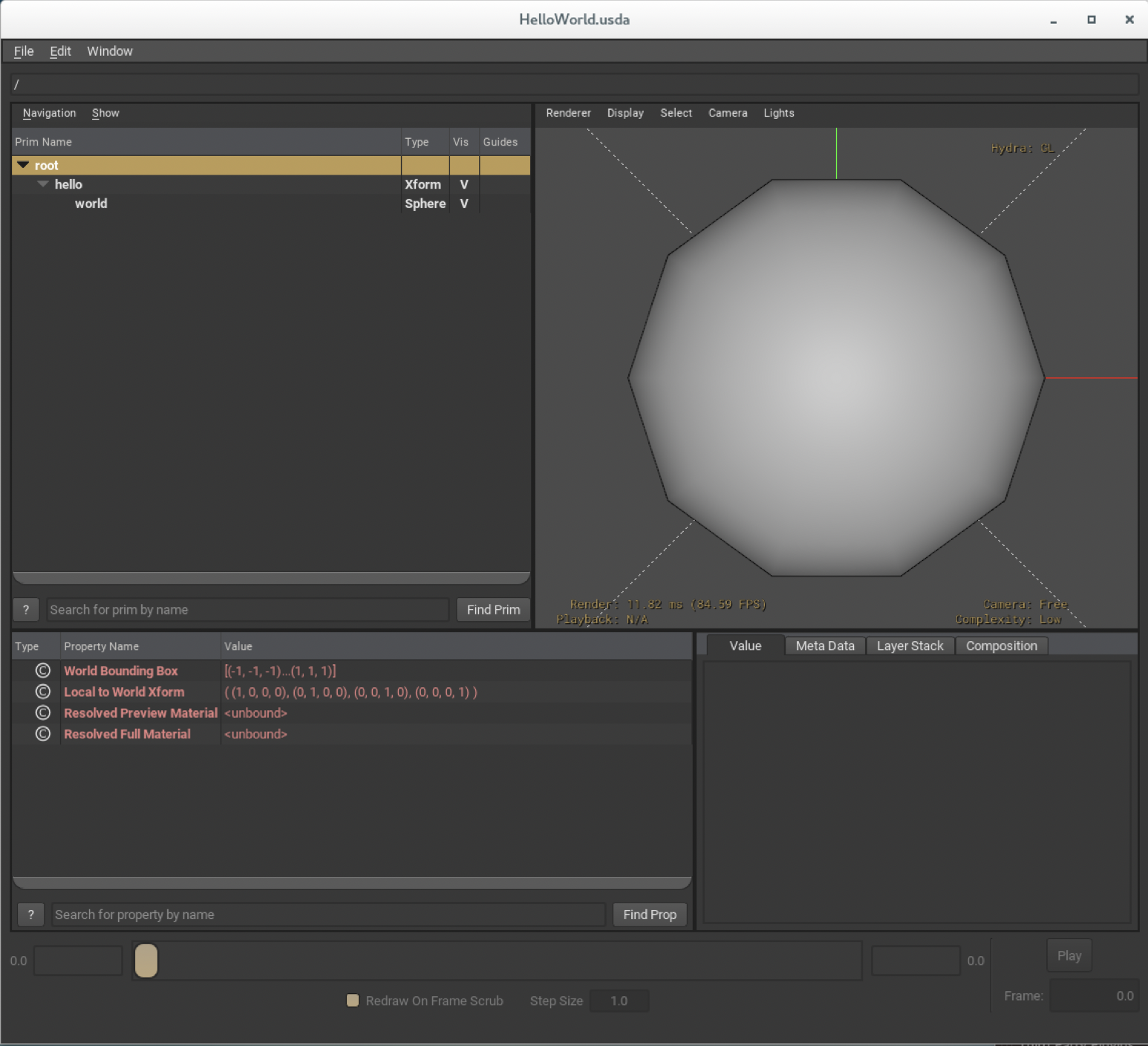
   

   

2. You can refine the geometry with the View ‣ Complexity menu item or use the hotkeys Ctrl-+ and Ctrl-- to increase or decrease the refinement.
   可以使用“视图”（View）“复杂度”（Complexity）菜单项优化几何体，或使用热键和来增加或减少优化。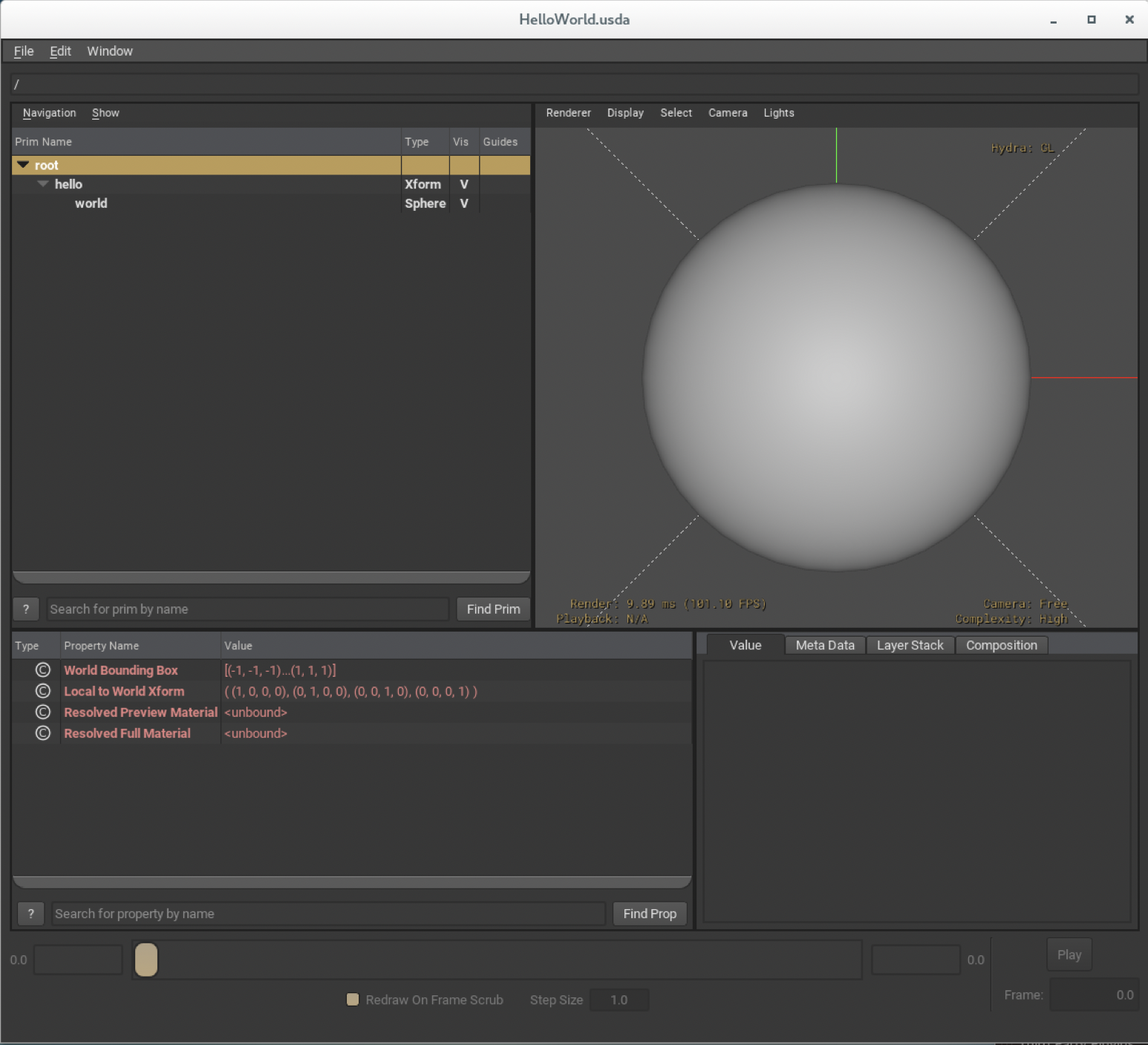

   

3. You can also bring up an embedded Python interpreter by pressing i or using the Window ‣ Interpreter menu item. This interpreter has a built-in API object, usdviewApi, that contains some useful variables. One is usdviewApi.prim, which refers to the first prim, hierarchically, in the set of currently selected prims.
   您还可以通过按下或使用Window Interpreter菜单项来调出嵌入式Python解释器。这个解释器有一个内置的API对象usdviewApi，它包含一些有用的变量。一个是usdviewApi.prim，它按层次结构引用当前选定prim集合中的第一个prim。

   Select the sphere either by clicking it in the viewport or by clicking its name, world, in the tree view on the left. Then try the following commands:
   通过在视口中单击球体或在左侧的树视图中单击其名称world来选择球体。然后尝试以下命令：

   >>> usdviewApi.prim
   Usd.Prim(</hello/world>)
   >>> usdviewApi.prim.GetTypeName()
   'Sphere'
   >>> usdviewApi.prim.GetAttribute('radius').Get()
   1.0
   

Viewing and editing USD file contents
查看和编辑USD文件内容

The exported file is human-readable via usdcat and text-editable via usdedit (both available in USD_INSTALL_ROOT/bin in the default installation). The usdedit program will bring up any .usd file as plain text in your EDITOR regardless of its underlying format, and save it back out in its original format when editing is complete. See usdedit for more details.
导出的文件可以通过usdcat读取，也可以通过usdedit进行文本编辑（默认安装中的USD_INSTALL_ROOT/bin中都有）。usdedit程序会在您的文件中以纯文本形式显示任何.usd文件，而不管其底层格式如何，并在编辑完成后以原始格式保存。查看usdedit了解更多详情。

This particular example can be edited in a text editor directly since we created a text-based USD file with the .usda extension. If we had created a binary usd file with the .usdc extension instead, both usdcat and usdedit would work just the same on it.
这个特殊的例子可以直接在文本编辑器中编辑，因为我们创建了一个基于文本的USD文件，扩展名为.usda。如果我们创建了一个扩展名为.usdc的二进制usd文件，usdcat和usdedit都可以在上面工作。

#usda 1.0

def Xform "hello"
{
    def Sphere "world"
    {
    }
}

Further Reading 进一步阅读

• UsdStage is the outermost container for scene description, which owns and presents composed prims as a scenegraph.
  UsdStage是场景描述的最外层容器，它拥有并将合成的prims呈现为scenegraph。

• UsdPrim is the sole persistent scenegraph object on a UsdStage.
  UsdPrim是UsdStage上唯一的持久性场景图对象。

Hello World Redux - Using Generic Prims
Hello World Redux -使用通用Prims

In this tutorial, we revisit the Hello World! example, but this example passes in hard-coded typenames Xform and Sphere, which correspond to the typenames appearing after the def specifiers in the usda scene description representation.
在本教程中，我们将重新访问Hello World！例如，但是这个例子传递了硬编码的类型名Xform和Sphere，它们对应于出现在usda场景描述表示中的def说明符之后的类型名。

The UsdGeom API used in the previous tutorial, is part of USD’s built-in geometry schema. These prim types and associated C++ and Python API have first-class support in USD and provide domain-specific interfaces to create, manipulate, introspect and author properties upon them.
上一个教程中使用的UsdGeom API是USD内置几何模式的一部分。这些prim类型和相关的C++和Python API在USD中具有一流的支持，并提供特定于域的接口来创建，操作，内省和作者属性。

Note that UsdGeomXform::Define returns a schema object on which the full schema-specific API is available, as opposed to UsdStage::DefinePrim which returns a generic UsdPrim. In USD, all schema classes have a GetPrim() member function that returns its underlying UsdPrim. Think of a UsdPrim as the object’s generic, persistent presence in the scenegraph, and the schema object as the first-class way to access its domain-specific data and functionality.
请注意，UsdGeomXform：：Define返回一个模式对象，在该对象上可以使用完整的特定于模式的API，而UsdStage：：DefinePrim返回一个通用的UsdPrim。在USD中，所有模式类都有一个GetPrim（）成员函数，该函数返回其基础UsdPrim。可以将UsdPrim看作是对象在场景图中的通用持久存在，而模式对象则是访问其特定于域的数据和功能的第一类方法。

from pxr import Usd
stage = Usd.Stage.CreateNew('HelloWorldRedux.usda')
xform = stage.DefinePrim('/hello', 'Xform')
sphere = stage.DefinePrim('/hello/world', 'Sphere')
stage.GetRootLayer().Save()

The code above produces identical scene description to the previous tutorial, which you can see using usdcat:
上面的代码生成了与上一个教程相同的场景描述，您可以使用usdcat看到：

#usda 1.0

def Xform "hello"
{
    def Sphere "world"
    {
    }
}

In the next tutorial, we’ll look at UsdGeom API in action on prim properties.
在下一个教程中，我们将研究UsdGeom API在prim属性上的作用。

Inspecting and Authoring Properties
检查和创作属性

In this tutorial we look at properties containing geometric data on the prims we created in the Hello World tutorial. The starting layer for this exercise is extras/usd/tutorials/authoringProperties/HelloWorld.usda.
在本教程中，我们将查看包含在Hello World教程中创建的prims上的几何数据的属性。本练习的起始图层是extras/usd/tutorials/authoringProperties/HelloWorld. usda。

This tutorial is available in extras/usd/tutorials/authoringProperties/authorProperties.py. You can follow along with this script in Python.
本教程位于extras/usd/tutorials/authoringProperties/authorProperty.py。你可以在Python中使用这个脚本。

Tutorial 教程

1. Open the stage and get the prims defined on the stage.
   打开舞台并获取舞台上定义的素数。

   from pxr import Usd, Vt
   stage = Usd.Stage.Open('HelloWorld.usda')
   xform = stage.GetPrimAtPath('/hello')
   sphere = stage.GetPrimAtPath('/hello/world')
   

2. List the available property names on each prim.
   列出每个prim上的可用特性名称。

   >>> xform.GetPropertyNames()
   ['proxyPrim', 'purpose', 'visibility', 'xformOpOrder']
   >>> sphere.GetPropertyNames()
   ['doubleSided', 'extent', 'orientation', 'primvars:displayColor',
   'primvars:displayOpacity', 'proxyPrim', 'purpose', 'radius',
   'visibility', 'xformOpOrder']
   

3. Read the extent attribute on the sphere prim.
   读取球体prim上的范围属性。

   >>> extentAttr = sphere.GetAttribute('extent')
   >>> extentAttr.Get()
   Vt.Vec3fArray(2, (Gf.Vec3f(-1.0, -1.0, -1.0), Gf.Vec3f(1.0, 1.0, 1.0)))
   

   This returns a two-by-three array containing the endpoints of the sphere’s axis-aligned, object-space extent, as expected for the fallback value of this attribute. An attribute has a fallback value when no opinions about its value are authored in the scene description. This fallback value for extent is sensible given that the fallback value for a sphere’s radius is 1.0.
   这将返回一个二乘三的数组，其中包含球体的轴对齐对象空间范围的端点，这与此属性的回退值所预期的一样。当场景描述中未编写有关属性值的意见时，属性具有回退值。如果球体半径的回退值为1.0，则此范围回退值是合理的。

   A call to Usd.Attribute.Get() with no arguments returns the attribute’s value at the Default time. Attributes can also have time-sampled values. For example, we can create an animated deforming object by providing time sample values for a UsdGeom.Mesh’s points attribute. (See End to End Example for a mock-up of this pipeline in action).
   不带参数地调用Usd.Attribute.Get（）将返回默认时间的属性值。属性也可以具有时间采样值。例如，我们可以通过为UsdGeom.Mesh的points属性提供时间采样值来创建动画变形对象。(See端到端示例，用于该管线的实际模型）。

   API Tip API头端

   UsdPrim::GetPropertyNames demonstrates that we can fetch properties by name. In practice, to iterate over a prim’s properties it is generally more convenient to use one of UsdPrim::GetProperties, UsdPrim::GetAttributes, or UsdPrim::GetRelationships. These return UsdProperty, UsdAttribute, and UsdRelationship objects that one can operate on directly.
   UsdPrim：：GetPropertyNames演示了我们可以通过名称获取属性。在实践中，要迭代prim的属性，通常使用UsdPrim：：GetProperties、UsdPrim：：GetAttributes或UsdPrim：：GetRelationships中的一个更方便。它们返回可直接操作的UsdProperty、UsdAttribute和UsdRelationship对象。

4. Set the sphere’s radius to 2.
   将球体的半径设置为2。

   Since geometric extents are not automatically recomputed, we must also update the sphere’s extent to reflect its new size. See more details here.
   由于几何范围不会自动重新计算，因此我们还必须更新球体的范围以反映其新大小。查看更多详情此处。

   >>> radiusAttr = sphere.GetAttribute('radius')
    >>> radiusAttr.Set(2)
   True
   >>> extentAttr.Set(extentAttr.Get() * 2)
   True
   

   Like Get(), a call to Set() with a value argument and no time argument authors the value at the Default time. The resulting scene description is:
   与Get（）类似，使用value参数而不使用time参数的Set（）调用在Default时间创建值。生成的场景描述为：

   >>> print(stage.GetRootLayer().ExportToString())
   #usda 1.0
   
   def Xform "hello"
   {
       def Sphere "world"
       {
           float3[] extent = [(-2, -2, -2), (2, 2, 2)]
           double radius = 2
       }
   }
   

5. Author a displayColor on the sphere.
   在球体上编写displayColor。

   As with Hello World Redux - Using Generic Prims, we can do so using the UsdGeom schema API. One benefit to this approach is that the first-class API hides the fact that the attribute’s raw name is primvars:displayColor. This frees client code from having to know that detail.
   与Hello World Redux - Using Generic Prims一样，我们可以使用UsdGeom模式API来实现。这种方法的一个好处是，第一类API隐藏了属性的原始名称是primvars：displayColor的事实。这使得客户端代码不必知道这些细节。

   >>> from pxr import UsdGeom
   >>> sphereSchema = UsdGeom.Sphere(sphere)
   >>> color = sphereSchema.GetDisplayColorAttr()
   >>> color.Set([(0,0,1)])
   True
   

   Note that the color value is a vector of triples. This is because the primvars:displayColor attribute can represent either a single color for the whole prim, or a color per prim element (e.g. mesh face). The resulting scene description is:
   请注意，颜色值是三元组的向量。这是因为primvars：displayColor属性可以表示整个prim的单个颜色，也可以表示每个prim元素的颜色（例如网格面）。生成的场景描述为：

   >>> print(stage.GetRootLayer().ExportToString())
   #usda 1.0
   
   def Xform "hello"
   {
       def Sphere "world"
       {
           float3[] extent = [(-2, -2, -2), (2, 2, 2)]
           color3f[] primvars:displayColor = [(0, 0, 1)]
           double radius = 2
       }
   }
   

6. Save your edits. 保存您的编辑。

   >>> stage.GetRootLayer().Save()
   

7. Here is the result in usdview.
   下面是usdview中的结果。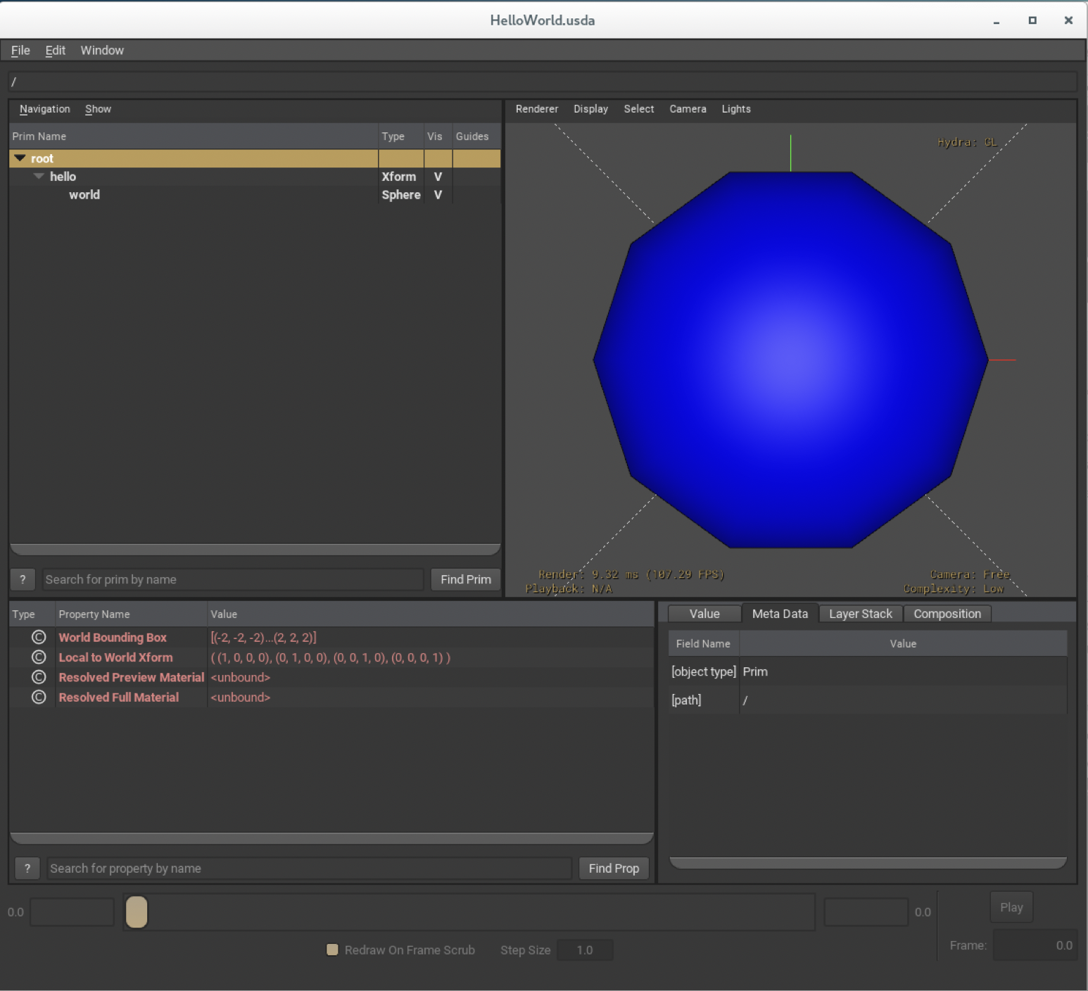

   

   The camera automatically frames the geometry, but we can see that the sphere is larger than in the last tutorial by inspecting its attributes in the Attribute browser.
   摄影机会自动框显几何体，但通过在“属性”（Attribute）浏览器中检查球体的属性，我们可以看到球体比上一个教程中的要大。

Further Reading 进一步阅读

• UsdProperty provides access to authoring and interrogating properties and their common metadata
  UsdProperty提供对创作和询问属性及其公共元数据的访问

• UsdAttribute refines UsdProperty with specific API for time-sampled access to typed attribute data
  UsdAttribute使用特定的API细化UsdProperty，以便对类型化属性数据进行时间采样访问

• UsdRelationship refines UsdProperty with API to target other prims and properties, and resolve those targets robustly, and through chains of relationships.
  UsdRelationship使用API细化UsdProperty以定位其他prims和属性，并通过关系链稳健地解析这些目标。

• Properties are ordered in dictionary order, by default, but one can explicitly order properties using UsdPrim::SetPropertyOrder.
  默认情况下，属性按字典顺序排序，但可以使用UsdPrim：：SetPropertyOrder显式地对属性进行排序。

   

Referencing Layers 参照层

This tutorial walks you through referencing the stage that we created in the previous tutorials into a new stage. The HelloWorld.usda that we will use as our starting point and all the code for this exercise is in the extras/usd/tutorials/referencingLayers folder.
本教程将引导您将在前面的教程中创建的舞台引用到新舞台中。我们将使用HelloWorld.usda作为我们的起点，本练习的所有代码都在extras/usd/tutorials/referencingLayers文件夹中。

1. Author the defaultPrim metadata on the layer that you want to reference. This is the name of the root prim that will be referenced. If it is not authored here, then the referencing client must specify the root prim path it wants from the referenced layer. We also want to author a transformation on the default root prim, so that we can override it later; to do this we use the UsdGeomXformCommonAPI schema, which we will discuss further, later.
   在要引用的图层上编写defaultPrim元数据。这是将要引用的根prim的名称。如果不是在此处创作的，则引用客户端必须指定它希望从引用层获得的根prim路径。我们还想在默认的根prim上创建一个转换，这样我们以后就可以覆盖它;为此，我们使用UsdGeomXformCommonAPI模式，稍后我们将进一步讨论。

   from pxr import Usd, UsdGeom
   stage = Usd.Stage.Open('HelloWorld.usda')
   hello = stage.GetPrimAtPath('/hello')
   stage.SetDefaultPrim(hello)
   UsdGeom.XformCommonAPI(hello).SetTranslate((4, 5, 6))
   print(stage.GetRootLayer().ExportToString())
   stage.GetRootLayer().Save()
   

   produces 产生

   #usda 1.0
   (
       defaultPrim = "hello"
   )
   
   def Xform "hello"
   {
       double3 xformOp:translate = (4, 5, 6)
       uniform token[] xformOpOrder = ["xformOp:translate"]
   
       def Sphere "world"
       {
           float3[] extent = [(-2, -2, -2), (2, 2, 2)]
           color3f[] primvars:displayColor = [(0, 0, 1)]
           double radius = 2
       }
   }
   

2. Now let’s create a new stage to reference in HelloWorld.usda and create an override prim to contain the reference.
   现在，让我们在HelloWorld.usda中创建一个新的阶段来引用，并创建一个覆盖prime来包含引用。

   refStage = Usd.Stage.CreateNew('RefExample.usda')
   refSphere = refStage.OverridePrim('/refSphere')
   print(refStage.GetRootLayer().ExportToString())
   

   produces 产生

   #usda 1.0
   
   over "refSphere"
   {
   }
   

   All of the previous prims we had created are def s , which are concrete prims that appear in standard scenegraph traversals (i.e. by clients performing imaging, or importing the stage into another DCC application). By contrast, an over can be thought of as containing a set of speculative opinions that are applied over any concrete prims that may be defined in other layers at the corresponding namespace location in a composed stage. Overs can contain opinions for any property, metadata, or prim composition operators. For example, an over can non-destructively express a different opinion for the transform and displayColor attributes above.
   我们之前创建的所有素数都是def s，它们是出现在标准场景图遍历中的具体素数（即客户端执行成像，或将载物台导入到另一DCC应用程序中）。相比之下，over可以被认为是包含一组推测性意见，这些意见被应用于可以在组合阶段中的对应命名空间位置处的其他层中定义的任何具体素数。Overs可以包含任何属性、元数据或prim组合操作符的意见。例如，over可以非破坏性地表达对上述transform和displayColor属性的不同意见。

3. Let’s reference in the stage from HelloWorld.
   让我们参考HelloWorld的阶段。

   refSphere.GetReferences().AddReference('./HelloWorld.usda')
   print(refStage.GetRootLayer().ExportToString())
   refStage.GetRootLayer().Save()
   

   produces 产生

   #usda 1.0
   
   over "refSphere" (
       prepend references = @./HelloWorld.usda@
   )
   {
   }
   

   Asset Path Resolver and File Format Plugins
   资源路径解析器和文件格式插件

   In this example we use a filename to reference the layer. In practice, the layer identifier passed to Usd.References.AddReference() can be any string that a path resolver plugin can resolve and a scene description file format plugin would process to populate the actual scene description. USD supports user-implementable asset path resolver and file format plugins to allow site-specific customization and pipeline integration. USD does not require that layers be files on disk. See the Ar library documentation for more about asset resolvers, and see the code in USD/extras/usd/examples/usdObj/ for an example file format plugin.
   在本例中，我们使用文件名来引用图层。在实践中，传递给Usd.References.AddReference（）的层标识符可以是路径解析器插件可以解析并且场景描述文件格式插件将处理以填充实际场景描述的任何字符串。USD支持用户可实现的资产路径解析器和文件格式插件，以允许特定于站点的自定义和管道集成。USD不要求图层是磁盘上的文件。有关资产解析器的更多信息，请参阅Ar库文档，并请参阅USD/extras/usd/examples/usdObj/中的代码，以获取示例文件格式插件。

   Note that since we authored defaultPrim in HelloWorld.usda, we only need to specify the root layer we want to reference, and it is inferred that we will be bringing in the scenegraph contents rooted at /hello into our /refSphere.
   注意，由于我们在HelloWorld.usda中编写了defaultPrim，我们只需要指定我们想要引用的根层，并且推断我们将把根在/hello的场景图内容引入到我们的/refSphere中。

   Running usdview on the exported RefExample.usda shows the composed result.
   对导出的RefExample.usda运行usdview将显示合成结果。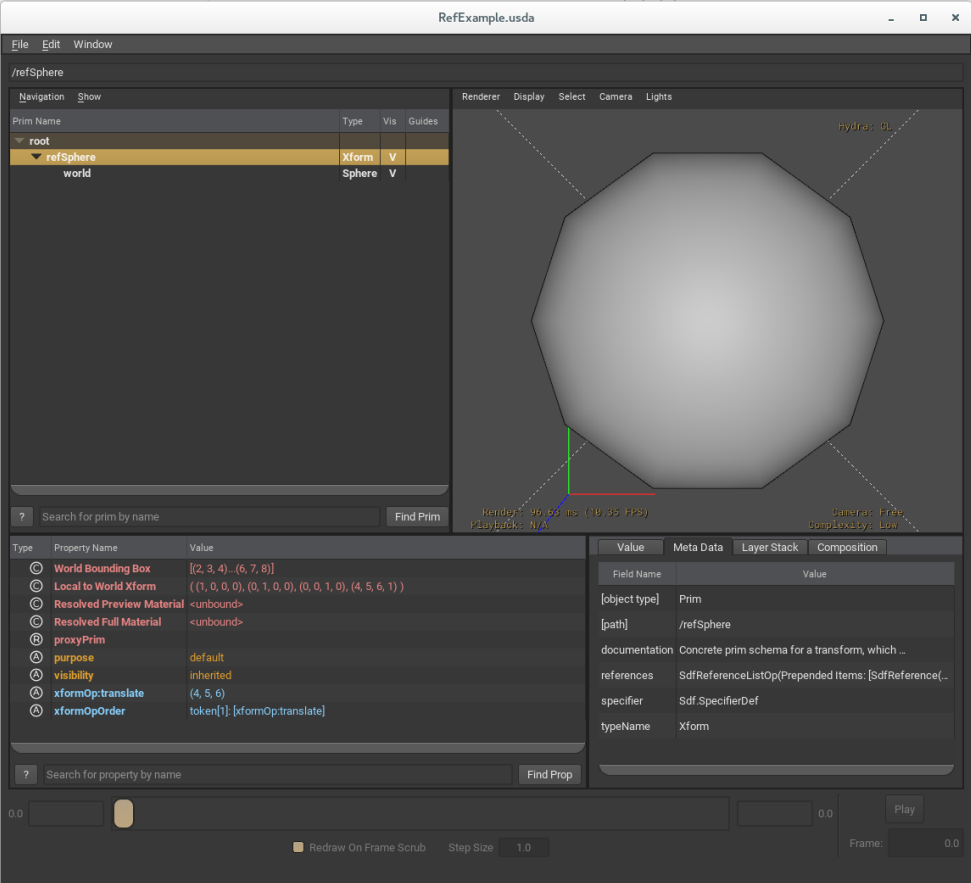

   

   If it were unselected in the namespace browser, usdview would show /refSphere in orange to indicate that it is a referencing point on our stage. Our screenshot shows refSphere’s row selected, however, to show both what our overridden transformation looks like as attributes, and to note in the Meta Data inspector that the reference and its target are listed. Note also that there is no prim named “hello” since it has been referenced into /refSphere.
   如果在名称空间浏览器中未选中它，usdview将以橙子显示/refSphere，以指示它是我们舞台上的引用点。我们的屏幕截图显示了refSphere的行被选中，但是，为了显示我们覆盖的转换作为属性的样子，并在Meta数据检查器中注意到引用及其目标被列出。还要注意，没有名为“hello”的prim，因为它已被引用到/refSphere中。

4. Let’s reset the transform on our over to the identity.
   让我们重新设置转换到恒等式。

   refXform = UsdGeom.Xformable(refSphere)
   refXform.SetXformOpOrder([])
   print(refStage.GetRootLayer().ExportToString())
   

   produces 产生

   #usda 1.0
   
   over "refSphere" (
       prepend references = @./HelloWorld.usda@
   )
   {
       uniform token[] xformOpOrder = []
   }
   

   What Just Happened? 第100章刚刚发生了什么？

   The UsdGeomXformable schema is component-based, allowing you to specify a single 4x4 matrix, or an unlimited sequence of translate, rotate, scale, matrix, and (quaternion) orientation “ops”. Each xformable prim has a builtin xformOpOrder attribute that specifies the order in which the ops are applied. By explicitly setting the ordering to an empty list as in:
   UsdGeomXformable模式是基于组件的，允许您指定单个4x 4矩阵，或无限制的平移、旋转、缩放、矩阵和（四元数）方向“操作”序列。每个可xformable prim都有一个内置的xformOpOrder属性，该属性指定操作的应用顺序。通过显式地将排序设置为空列表，如下所示：

   refXform.SetXformOpOrder([])
   refXform. SetXformOpOrder（[]）（英文）

   we are telling the schema to ignore any ops, even if authored, effectively setting the transformation to the identity. We could also have explicitly authored an identity matrix, or set all existing, composed op attributes to their identity values. For a complete explanation of Xformable and XformOps, please see the API documentation for UsdGeomXformable
   我们正在告诉模式忽略任何op，即使是编写的，有效地将转换设置为标识。我们还可以显式地创建一个单位矩阵，或者将所有现有的组合op属性设置为它们的单位值。有关Xformable和XformOps的完整说明，请参阅UsdGeomXformable的API文档

5. Reference in another HelloWorld.
   在另一个HelloWorld中引用。

   refSphere2 = refStage.OverridePrim('/refSphere2')
   refSphere2.GetReferences().AddReference('./HelloWorld.usda')
   print(refStage.GetRootLayer().ExportToString())
   refStage.GetRootLayer().Save()
   

   produces 产生

   #usda 1.0
   
   over "refSphere" (
       prepend references = @./HelloWorld.usda@
   )
   {
       uniform token[] xformOpOrder = []
   }
   
   over "refSphere2" (
       prepend references = @./HelloWorld.usda@
   )
   {
   }
   

   

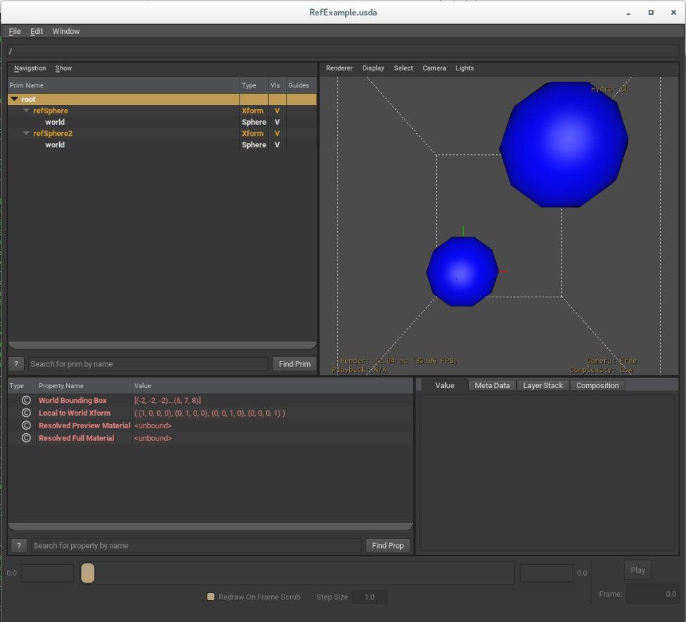
   We can see that our over has been applied to move the first sphere to the origin, while the second sphere is still translated by (4, 5, 6).
   我们可以看到，我们的翻转已经被应用到移动第一个球体到原点，而第二个球体仍然平移（4，5，6）。

6. Of course, overs can be authored for the actual sphere prims underneath the reference as well. Let’s color our second sphere red.
   当然，也可以为参照下面的实际球体素数编写覆盖。让我们把第二个球体涂成红色。

   overSphere = UsdGeom.Sphere.Get(refStage, '/refSphere2/world')
   overSphere.GetDisplayColorAttr().Set( [(1, 0, 0)] )
   print(refStage.GetRootLayer().ExportToString())
   refStage.GetRootLayer().Save()
   

   Note that we don’t need to call OverridePrim again because /refSphere2/world already has a presence in the composed scenegraph. USD automatically creates an over when Usd.Attribute.Set() is called if one doesn’t already exist for that prim in the current authoring layer.
   请注意，我们不需要再次调用OverridePrim，因为/refSphere 2/world已经存在于合成的场景图中。当调用Usd.Attribute.Set（）时，如果当前创作层中该prim还不存在，则USD会自动创建over。

   #usda 1.0
   
   over "refSphere" (
       prepend references = @./HelloWorld.usda@
   )
   {
       uniform token[] xformOpOrder = []
   }
   
   over "refSphere2" (
       prepend references = @./HelloWorld.usda@
   )
   {
       over "world"
       {
           color3f[] primvars:displayColor = [(1, 0, 0)]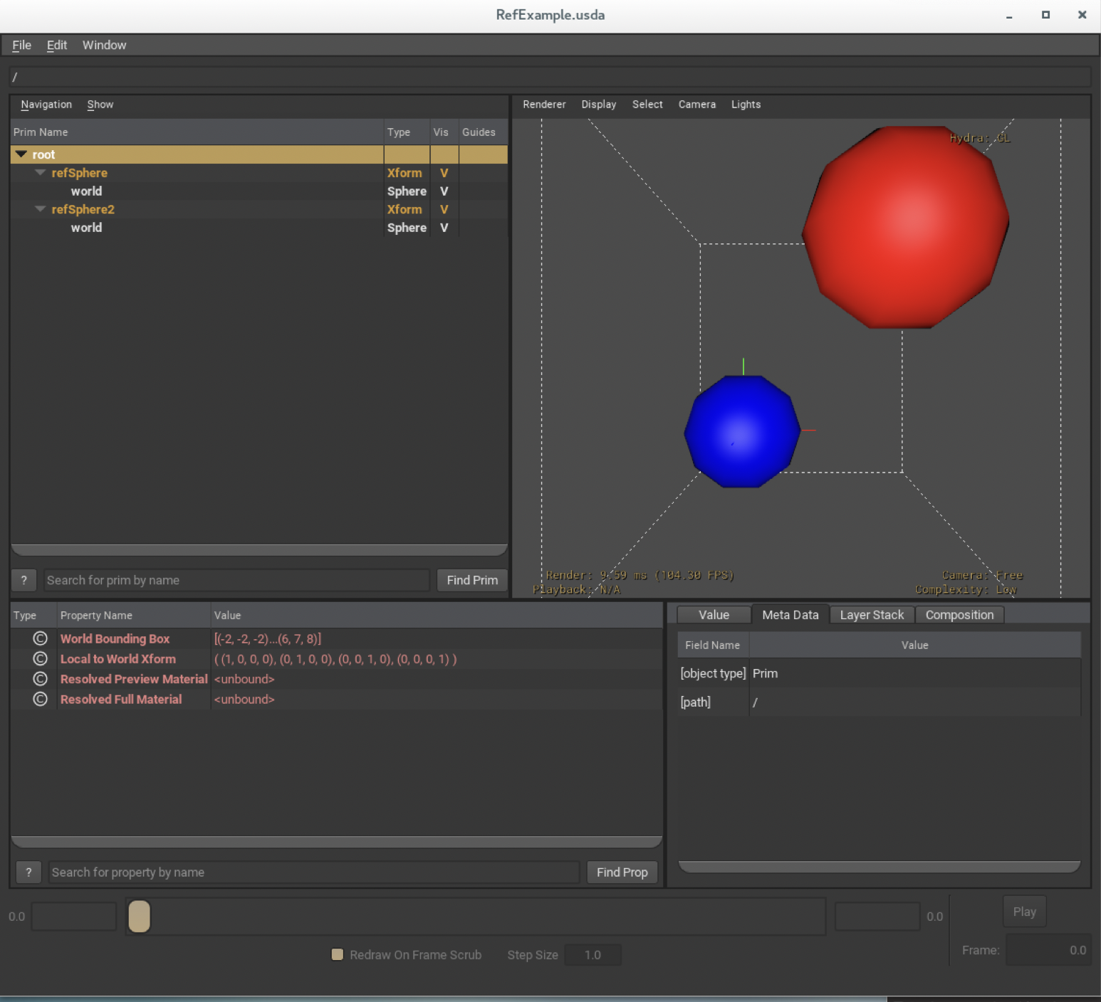
       }
   }
   

   

7. We can also flatten the composed results. All of the scene description listings above were of the stage’s root layer, where we performed our authoring. Calling ExportToString() or Export() on the UsdStage itself, will print or save out flattened scene description, respectively.
   我们还可以使合成结果平坦化。上面列出的所有场景描述都是舞台的根层，我们在这里进行创作。在UsdStage本身上调用ExportToString（）或Export（）将分别打印或保存展平的场景描述。

   flattening 展平

   The term flattening generally means producing a single Layer of scene description that contains the final “composed data” from a set of composed layers, and retains no composition operators such as references, payloads, inherits, variants, sublayers, and activations (except references generated in order to preserve scene graph instancing). UsdStage::Flatten flattens an entire stage and is used by Export() and ExportToString(). USD also supports flattening individual layer stacks. See UsdFlattenLayerStack.
   术语扁平化通常意味着产生场景描述的单个层，其包含来自一组合成层的最终“合成数据”，并且不保留合成操作符，诸如引用、有效载荷、继承、变体、子层和激活（除了为了保留场景图实例化而生成的引用之外）。UsdStage：：Flatten拼合整个舞台，并由Export（）和ExportToString（）使用。USD还支持扁平化单个层堆栈。请参见UsdFlattenLayerStack。

   print(refStage.ExportToString())
   

   #usda 1.0
   (
       doc = """Generated from Composed Stage of root layer RefExample.usda
   """
   )
   
   def Xform "refSphere"
   {
       double3 xformOp:translate = (4, 5, 6)
       uniform token[] xformOpOrder = []
   
       def Sphere "world"
       {
           float3[] extent = [(-2, -2, -2), (2, 2, 2)]
           color3f[] primvars:displayColor = [(0, 0, 1)]
           double radius = 2
       }
   }
   
   def Xform "refSphere2"
   {
       double3 xformOp:translate = (4, 5, 6)
       uniform token[] xformOpOrder = ["xformOp:translate"]
   
       def Sphere "world"
       {
           float3[] extent = [(-2, -2, -2), (2, 2, 2)]
           color3f[] primvars:displayColor = [(1, 0, 0)]
           double radius = 2
       }
   }

   Converting Between Layer Formats
   在图层格式之间转换

   This tutorial walks through converting layer files between the different native USD file formats.
   本教程将介绍如何在不同的原生USD文件格式之间转换图层文件。

   The usdcat tool is useful for inspecting these files, but it can also convert files between the different formats by using the -o option and supplying a filename with the extension of the desired output format. Here are some examples of how to do this.
   usdcat工具对于检查这些文件非常有用，但它也可以通过使用选项并提供带有所需输出格式扩展名的文件名来在不同格式之间转换文件。下面是一些如何做到这一点的例子。

   Converting between .usda/.usdc and .usd
   .usda/.usdc和.usd之间的转换

   A .usd file can be either a text or binary format file. When USD opens a .usd file, it detects the underlying format and handles the file appropriately. You can convert any .usda or .usdc file to a .usd file simply by renaming it. For example:
   .usd文件可以是文本或二进制格式的文件。当USD打开.usd文件时，它会检测基础格式并适当处理该文件。您可以将任何.usda或.usdc文件转换为.usd文件，只需重命名即可。举例来说：

   Given Sphere.usda, you can simply rename it to Sphere.usd.
   给定Sphere.usda，您可以简单地将其重命名为Sphere. usd。

   • When USD opens Sphere.usd, it detects that it uses the text file format and opens it appropriately. This works similarly for .usdc files.
     当USD打开Sphere.usd时，它会检测到它使用的是文本文件格式，并正确地打开它。这对.usdc文件的作用类似。

   A Sphere.usd file that uses the text format can be renamed to Sphere.usda
   使用文本格式的Sphere.usd文件可以重命名为Sphere.usda

   A Sphere.usd file that uses the binary format can be renamed to Sphere.usdc.
   使用二进制格式的Sphere.usd文件可以重命名为Sphere. usdc。

   Convert a binary .usd file to a text .usd the same way:
   将二进制.usd文件转换为文本.usd的方法相同：

   $ usdcat -o NewSphere_text.usd --usdFormat usda NewSphere_binary.usd
   $ usddiff NewSphere_binary.usd NewSphere_text.usd

   Converting between .usda and .usdc Files
   在.usda和.usdc文件之间转换

   Consider Sphere.usda in USD/extras/usd/tutorials/convertingLayerFormats. This is a text format file, so it can be examined in any text editor or via usdcat.
   考虑美元/extras/usd/tutorials/convertingLayerFormats中的Spher.usda。这是一个文本格式文件，因此可以在任何文本编辑器中或通过usdcat检查它。

   $ usdcat Sphere.usda
   
   #usda 1.0
   def Sphere "sphere"
   {
   }
   

   To convert this file to binary, we can specify an output filename with the .usdc extension:
   要将此文件转换为二进制文件，我们可以指定一个带有.usdc扩展名的输出文件名：

   $ usdcat -o NewSphere.usdc Sphere.usda
   

   This produces a binary file named Sphere.usdc in the current directory containing the same content as Sphere.usda. We can verify this using usddiff:
   这将在当前目录中生成一个名为Sphere.usdc的二进制文件，其中包含与Sphere. usda相同的内容。我们可以使用usddiff来验证这一点：

   $ usddiff Sphere.usda NewSphere.usdc
   

   Converting binary to text can be done the same way:
   将二进制文件转换为文本可以通过相同的方式完成：

   $ usdcat -o NewSphere.usda NewSphere.usdc
   $ usddiff NewSphere.usdc NewSphere.usda
   

   Converting between .usd Files of Different Formats
   在不同格式的.usd文件之间转换

   Note 注记

   If you have a .usda or .usdc file and want to make it a .usd file without changing the underlying format, you do not need to use usdcat; just rename the file. See Converting between .usda/.usdc and .usd above.
   如果您有一个.usda或.usdc文件，并希望在不更改基础格式的情况下将其变为.usd文件，则不需要使用usdcat;重命名文件即可。请参阅上面的.usda/.usdc和.usd之间的转换。

   If you have a .usd file of a particular format and want to convert it to a .usd file using a different format, pass the --usdFormat option to usdcat. Starting with Sphere.usd in USD/extras/usd/tutorials/convertingLayerFormats, which is a text format file, we can converty to a binary format file:
   如果您有特定格式的.usd文件，并希望将其转换为使用其他格式的.usd文件，请将该选项传递给usdcat。从USD/extras/usd/tutorials/convertingLayerFormats中的Sphere.usd开始，这是一个文本格式文件，我们可以转换为二进制格式文件：

   $ usdcat -o NewSphere_binary.usd --usdFormat usdc Sphere.usd
   

   We can verify the two files match:
   我们可以验证这两个文件是否匹配：

   $ usddiff Sphere.usd NewSphere_binary.usd
   

   Traversing a Stage 穿越舞台

   This tutorial covers API for traversing the composed prims on a UsdStage. This is the typical pattern for implementing imaging clients, USD importers to other DCC applications, etc. We will use the layers produced in Referencing Layers. You will need the referenced layer, HelloWorld.usda, and the referencing layer, RefExample.usda, which are in the USD/extras/usd/tutorials/traversingStage folder. Please copy that folder to a working directory and make its contents writable.
   本教程介绍用于在UsdStage上遍历合成prim的API。这是实现映像客户端、其他DCC应用程序的USD导入程序等的典型模式。我们将使用在参考层中生成的层。您需要参考层HelloWorld.usda和参考层RefExample.usda，它们位于USD/extras/usd/tutorials/traversingStage文件夹中。请将该文件夹复制到工作目录并使其内容可写。

   Open RefExample.usda in usdview and bring up the interpreter by hitting i or the Window ‣ Interpreter menu item.
   在usdview中打开RefExample.usda，点击或Window Interpreter菜单项，调出解释器。

   The interpreter has a built-in usdviewApi object that contains a number of convenient variables and functions for working with usdview and the UsdStage it has open.
   解释器有一个内置的usdviewApi对象，其中包含许多方便的变量和函数，用于处理usdview和它打开的UsdStage。

   The simplest place to start is with Usd.Stage.Traverse(); a generator which yields prims from the stage in depth-first-traversal order.
   最简单的起点是Usd.Stage.Traverse（）;生成器，其以深度优先遍历顺序从所述级产生素数。

   >>> [x for x in usdviewApi.stage.Traverse()]
   [Usd.Prim(</refSphere>), Usd.Prim(</refSphere/world>),
    Usd.Prim(</refSphere2>), Usd.Prim(</refSphere2/world>)]
   

   You can filter as you would any other Python generator:
   你可以像其他Python生成器一样过滤：

   >>> [x for x in usdviewApi.stage.Traverse() if UsdGeom.Sphere(x)]
   [Usd.Prim(</refSphere/world>), Usd.Prim(</refSphere2/world>)]
   

   For more involved traversals, the Usd.PrimRange() exposes pre- and post-order prim visitations.
   对于更复杂的遍历，Usd.PrimRange（）公开了顺序前和顺序后的prim访问。

   >>> primIter = iter(Usd.PrimRange.PreAndPostVisit(usdviewApi.stage.GetPseudoRoot()))
   >>> for x in primIter: print(x, primIter.IsPostVisit())
   Usd.Prim(</>) False
   Usd.Prim(</refSphere>) False
   Usd.Prim(</refSphere/world>) False
   Usd.Prim(</refSphere/world>) True
   Usd.Prim(</refSphere>) True
   Usd.Prim(</refSphere2>) False
   Usd.Prim(</refSphere2/world>) False
   Usd.Prim(</refSphere2/world>) True
   Usd.Prim(</refSphere2>) True
   Usd.Prim(</>) True
   

   Usd.PrimRange also makes prim-flag predicates available. In fact, Usd.Stage.Traverse() is really a convenience method that performs pre-order visitations on all the prims in the composed scenegraph that are active, defined, loaded, and concrete.
   Usd.PrimRange还使prim-flag谓词可用。事实上，Usd.Stage.Traverse（）确实是一个方便的方法，它可以对组合场景图中所有活动的、已定义的、已加载的和具体的元素执行预排序访问。

   In Referencing Layers, we touched upon what it means for a prim to be defined, i.e., it is backed by a def rather than an over. The concepts of being loaded and concrete respectively correlate to payloads (composition boundaries across which scene description does not get composed unless explicitly requested) and classes (abstract prims whose opinions apply to all prims which inherit from them). We will discuss these operators more in depth in a future tutorial. Here we consider activation/deactivation semantics with usdview.
   在引用层中，我们触及了定义prim的含义，即，它由def而不是over支持。被加载和具体的概念分别与有效载荷（除非明确请求，否则场景描述不会跨越其组合的组合边界）和类（抽象素数，其意见适用于从它们继承的所有素数）相关。我们将在以后的教程中更深入地讨论这些运算符。这里我们考虑usdview的激活/停用语义。

   Select refSphere2 in the tree view on the left and choose Edit ‣ Deactivate from the menu. The result should look like this.
   在左侧的树视图中选择refSphere 2，然后从菜单中选择Edit Deactivate。结果应该如下所示。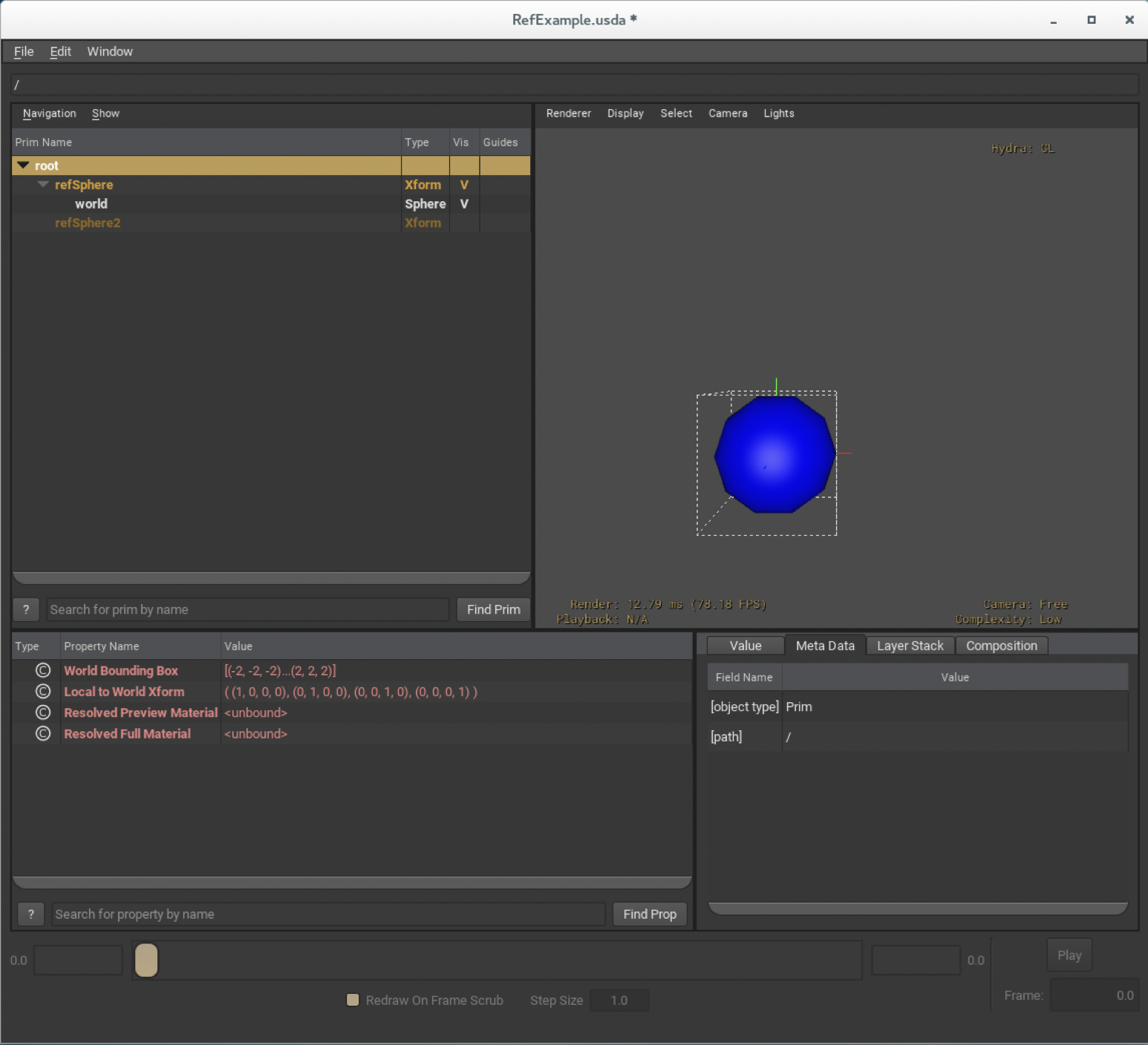

    

   

   You can inspect the contents of the session layer in the interpreter to see the authored deactivation opinion.
   您可以在解释器中检查会话层的内容，以查看创作的停用意见。

   >>> print(usdviewApi.stage.GetSessionLayer().ExportToString())
   #usda 1.0
   
   over "refSphere2" (
       active = false
   )
   {
   }
   

   In USD, a session layer holds transient opinions for the current working session that a user would not want to commit to the asset and thereby affect downstream departments.
   在USD中，会话层为当前工作会话保存用户不希望提交给资产并因此影响下游部门的瞬时意见。

   Now Traverse() will not visit refSphere2 or any of its namespace children, and renderers do not draw it.
   现在，Traverse（）将不会访问refSphere2或它的任何名称空间子对象，渲染器也不会绘制它。

   >>> [x for x in usdviewApi.stage.Traverse()]
   [Usd.Prim(</refSphere>), Usd.Prim(</refSphere/world>)]
   

   While we can still see refSphere2 as an inactive prim on the stage, its children no longer have any presence in the composed scenegraph. We can use TraverseAll() to get an iterator with no predicates applied to verify this.
   虽然我们仍然可以看到refSphere2在舞台上是一个不活跃的prim，但它的子节点在合成的场景图中不再存在。我们可以使用TraverseAll（）来获取一个迭代器，它没有应用任何谓词来验证这一点。

   >>> [x for x in usdviewApi.stage.TraverseAll()]
   [Usd.Prim(</refSphere>), Usd.Prim(</refSphere/world>),
    Usd.Prim(</refSphere2>)]

    

   Authoring Variants 编写变体

   This tutorial walks through authoring a variant set on the HelloWorld layer from Inspecting and Authoring Properties. We begin with the layer USD/extras/usd/tutorials/authoringVariants/HelloWorld.usda and the Python code authorVariants.py in the same directory. Please copy these files to a working directory and make them writable.
   本教程将从“检查和编写属性”中逐步在HelloWorld图层上编写变体集。我们从USD/extras/usd/tutorials/authoringVariants/HelloWorld.usda层和同一目录中的Python代码authorVariants.py开始。请将这些文件复制到一个工作目录并使其可写。

   1. Open the stage and clear the Sphere’s authored displayColor opinion. In USD local opinions are stronger than variant opinions. So if we do not clear this opinion it will win over those we author within variants below.
      打开舞台并清除Sphere的创作显示颜色意见。在美元中，本地意见比不同意见更强。因此，如果我们不明确这个观点，它将赢得我们在下面的变体中作者的支持。

      To see this in action, comment out the Clear() and run the tutorial. The steps below still author the same variant opinions, but the composed result shows the locally-authored blue color. That stronger local opinion overrides the opinions from variants.
      要查看实际操作，请注释掉Clear（）并运行教程。下面的步骤仍然创作相同的变体意见，但合成的结果显示本地创作的蓝色。这种更强烈的地方意见压倒了来自变体的意见。

      See LIVRPS Strength Ordering for more details on strength order in USD.
      请参阅LIVRPS强度订购以美元计价的更多详情。

      from pxr import Usd, UsdGeom
      stage = Usd.Stage.Open('HelloWorld.usda')
      colorAttr = UsdGeom.Gprim.Get(stage, '/hello/world').GetDisplayColorAttr()
      colorAttr.Clear()
      print(stage.GetRootLayer().ExportToString())
      

      The </hello/world> prim is a Sphere; a schema subclass of Gprim. So we can use the UsdGeom.Gprim API to work with it. In USD, Gprim defines displayColor so all gprim subclasses have it.
      prim是一个球体; Gprim的一个模式子类。所以我们可以使用UsdGeom.Gprim API来处理它。在USD中，Gprim定义了displayColor，因此所有gprim子类都有它。

      #usda 1.0
      (
          defaultPrim = "hello"
      )
      
      def Xform "hello"
      {
          custom double3 xformOp:translate = (4, 5, 6)
          uniform token[] xformOpOrder = ["xformOp:translate"]
      
          def Sphere "world"
          {
              float3[] extent = [(-2, -2, -2), (2, 2, 2)]
              color3f[] primvars:displayColor
              double radius = 2
          }
      }
      

      The resulting scene description still has the declaration for the displayColor attribute; a future iteration on the Usd.Attribute API may clean this up.
      生成的场景描述仍然具有displayColor属性的声明; Usd.Attribute API上的将来迭代可能会清除这个问题。

   2. Create a shading variant on the root prim called shadingVariant
      在根prim上创建一个名为shadingVariant的着色变体

      rootPrim = stage.GetPrimAtPath('/hello')
      vset = rootPrim.GetVariantSets().AddVariantSet('shadingVariant')
      print(stage.GetRootLayer().ExportToString())
      

      produces 产生

      #usda 1.0
      (
          defaultPrim = "hello"
      )
      
      def Xform "hello" (
          prepend variantSets = "shadingVariant"
      )
      {
          custom double3 xformOp:translate = (4, 5, 6)
          uniform token[] xformOpOrder = ["xformOp:translate"]
      
          def Sphere "world"
          {
              float3[] extent = [(-2, -2, -2), (2, 2, 2)]
              color3f[] primvars:displayColor
              double radius = 2
          }
      }
      

   3. Create variants within ‘shadingVariant’ to contain the opinions we will author.
      在'shadingVariant'中创建变体，以包含我们将要创作的观点。

      vset.AddVariant('red')
      vset.AddVariant('blue')
      vset.AddVariant('green')
      print(stage.GetRootLayer().ExportToString())
      

      produces 产生

      #usda 1.0
      (
          defaultPrim = "hello"
      )
      
      def Xform "hello" (
          prepend variantSets = "shadingVariant"
      )
      {
          custom double3 xformOp:translate = (4, 5, 6)
          uniform token[] xformOpOrder = ["xformOp:translate"]
      
          def Sphere "world"
          {
              float3[] extent = [(-2, -2, -2), (2, 2, 2)]
              color3f[] primvars:displayColor
              double radius = 2
          }
      
          variantSet "shadingVariant" = {
              "blue" {
              }
      
              "green" {
              }
      
              "red" {
              }
          }
      }
      

   4. Author a red color to the sphere prim </hello/world> in the red variant.
      为红色变体中的球体prim 创作一个红色。

      To author opinions inside the red variant we first select the variant, then use a Usd.EditContext. This directs editing into the variant.
      要在红色变体中创作观点，我们首先选择变体，然后使用Usd. EditContext。这引导编辑到变体中。

      vset.SetVariantSelection('red')
      with vset.GetVariantEditContext():
          colorAttr.Set([(1,0,0)])
      
      print(stage.GetRootLayer().ExportToString())
      

      If we just invoked colorAttr.Set() without using the variant edit context, we would write a local opinion; specifically the same opinion we cleared at the beginning.
      如果我们只调用colorAttr.Set（）而不使用变体编辑上下文，我们将编写一个本地意见;特别是我们一开始就澄清的意见

      #usda 1.0
      (
          defaultPrim = "hello"
      )
      
      def Xform "hello" (
          variants = {
              string shadingVariant = "red"
          }
          prepend variantSets = "shadingVariant"
      )
      {
          custom double3 xformOp:translate = (4, 5, 6)
          uniform token[] xformOpOrder = ["xformOp:translate"]
      
          def Sphere "world"
          {
              float3[] extent = [(-2, -2, -2), (2, 2, 2)]
              color3f[] primvars:displayColor
              double radius = 2
          }
      
          variantSet "shadingVariant" = {
              "blue" {
              }
      
              "green" {
              }
      
              "red" {
                  over "world"
                  {
                      color3f[] primvars:displayColor = [(1, 0, 0)]
                  }
              }
          }
      }
      

      Now hello has a shadingVariant with a default variant selection of red, and the red variant has an opinion for displayColor.
      现在hello有一个shadingVariant，默认变量选择为红色，红色变量有一个关于displayColor的意见。

   5. Author the blue and green variants similarly.
      同样地编写蓝色和绿色变体。

      vset.SetVariantSelection('blue')
      with vset.GetVariantEditContext():
          colorAttr.Set([(0,0,1)])
      
      vset.SetVariantSelection('green')
      with vset.GetVariantEditContext():
          colorAttr.Set([(0,1,0)])
      
      print(stage.GetRootLayer().ExportToString())
      

      produces 产生

      #usda 1.0
      (
          defaultPrim = "hello"
      )
      
      def Xform "hello" (
          variants = {
              string shadingVariant = "green"
          }
          prepend variantSets = "shadingVariant"
      )
      {
          custom double3 xformOp:translate = (4, 5, 6)
          uniform token[] xformOpOrder = ["xformOp:translate"]
      
          def Sphere "world"
          {
              float3[] extent = [(-2, -2, -2), (2, 2, 2)]
              color3f[] primvars:displayColor
              double radius = 2
          }
      
          variantSet "shadingVariant" = {
              "blue" {
                  over "world"
                  {
                      color3f[] primvars:displayColor = [(0, 0, 1)]
                  }
              }
      
              "green" {
                  over "world"
                  {
                      color3f[] primvars:displayColor = [(0, 1, 0)]
                  }
              }
      
              "red" {
                  over "world"
                  {
                      color3f[] primvars:displayColor = [(1, 0, 0)]
                  }
              }
          }
      }
      

      As mentioned at the beginning, it was important to first Clear() the local opinion for primvars:displayColor because local opinions are strongest. Had we not cleared the local opinion, the sphere would remain blue regardless of the selected shadingVariant for this reason.
      正如开头提到的，首先Clear（）primvars：displayColor的局部意见很重要，因为局部意见最强。如果我们没有清除局部意见，则球体将保持蓝色，而不考虑选择的shadingVariant。

      Opinion Strength Order 意见强度顺序

      Strength order is a fundamental part of USD.
      强势订单是美元的基本组成部分。

   6. Examine the composed result.
      检查合成结果。

      print(stage.ExportToString(addSourceFileComment=False))
      

      shows 展示

      #usda 1.0
      (
          defaultPrim = "hello"
      )
      
      def Xform "hello"
      {
          custom double3 xformOp:translate = (4, 5, 6)
          uniform token[] xformOpOrder = ["xformOp:translate"]
      
          def Sphere "world"
          {
              float3[] extent = [(-2, -2, -2), (2, 2, 2)]
              color3f[] primvars:displayColor = [(0, 1, 0)]
              double radius = 2
          }
      
      }
      

      What happened to the variants? Exporting a UsdStage writes the composed scene description with all the composition operators (like variants) fully evaluated. We call this flattening. Flattening the composition applies the opinions from the currently selected variants so we only get the green color due to the last call to SetVariantSelection().
      变种怎么了？导出UsdStage时，将写入所有合成操作符（如变体）完全求值的合成场景描述。我们称之为扁平化。展平组合会应用当前选择的变体的意见，因此我们只得到绿色，因为上次调用SetVariantSelection（）。

   7. Save the edited authoring layer to a new file, HelloWorldWithVariants.usda
      将编辑的创作层保存到新文件HelloWorldWithVariants.usda

      In contrast to exporting a UsdStage, exporting an individual layer writes its contents as-is to a different file. There is no flattening.
      与导出UsdStage相反，导出单个图层时会将其内容按原样写入不同的文件。没有变平。

      stage.GetRootLayer().Export('HelloWorldWithVariants.usda')
      

      We could also call Save() to update the original file with the new content.
      我们还可以调用保存（）来更新原始文件与新内容。

   8. Run usdview on HelloWorldWithVariants.usda.
      在HelloWorldWithVariants.usda上运行usdview。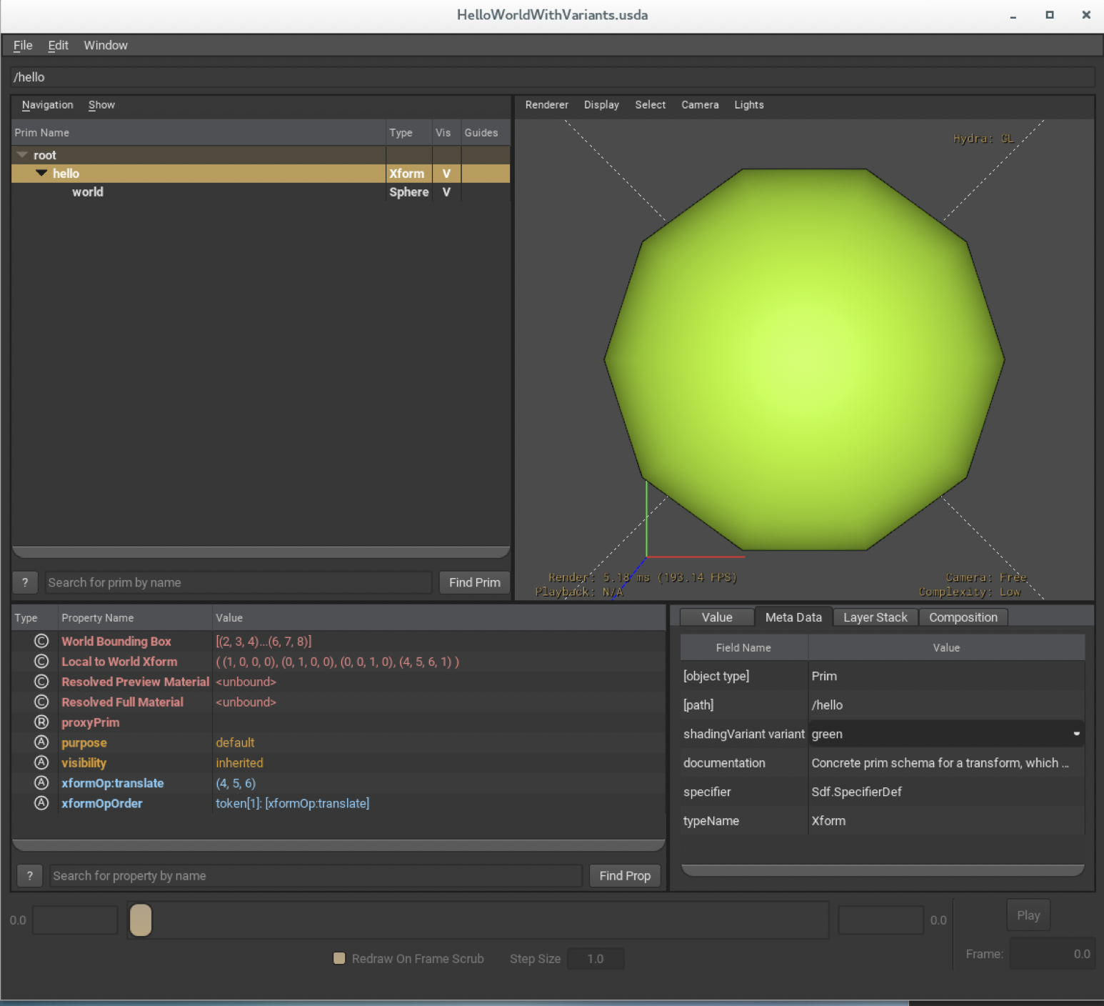

      

      Click the hello prim in the tree view on the left. Then click the Meta Data tab in the lower right. You will see the authored variant set with a combo box that can toggle the variant selection between red, blue, and green.
      单击左侧树视图中的hello prim。然后单击右下角的Meta数据选项卡。您将看到编写的变量集，其中包含一个组合框，可以在红色、蓝色和绿色之间切换变量选择。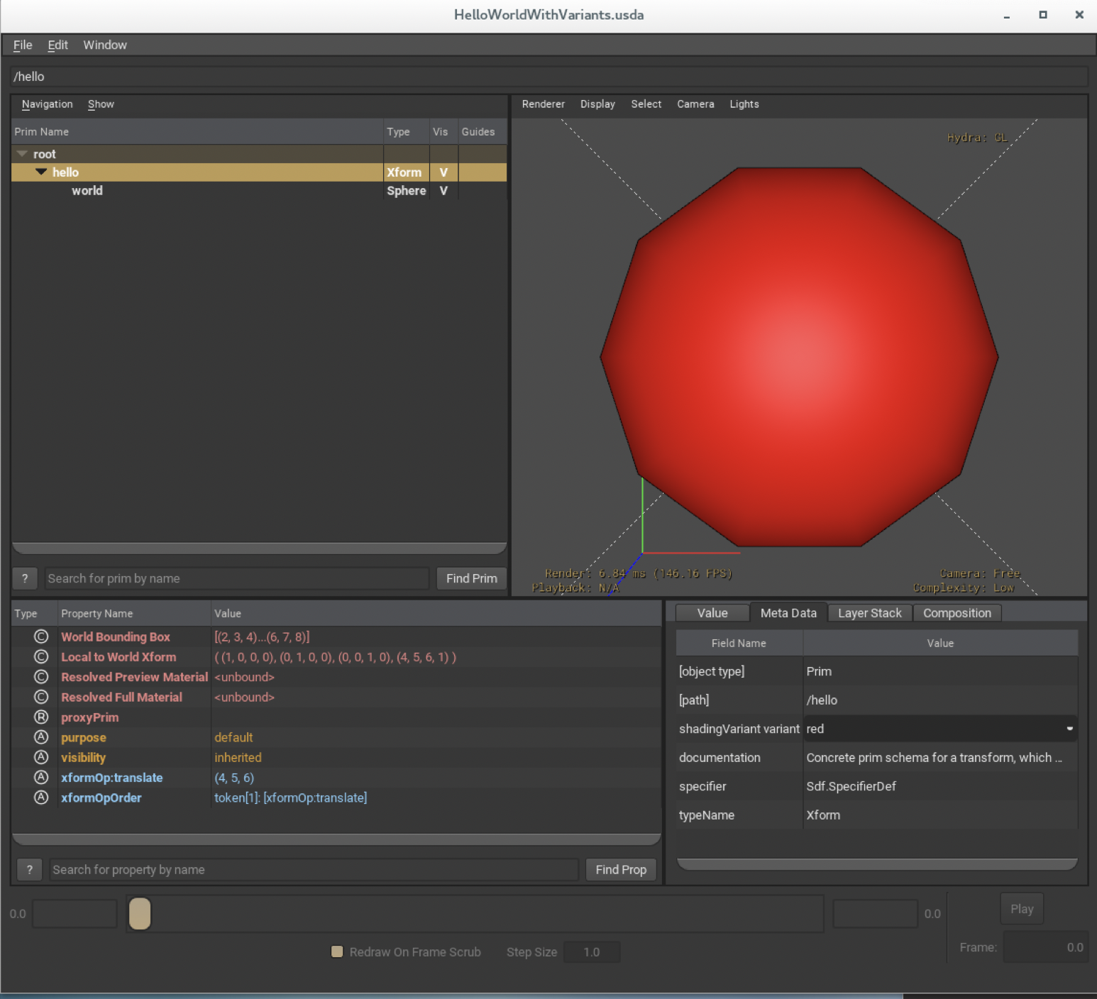

      

   9. In the interpreter you can see the variant selections that usdview authors to the session layer . This is the same sparse override you would see if you referenced this layer into another one and authored the variant selection in the referencing layer.
      在解释器中，您可以看到usdview创建到会话层的变量选择。如果将此图层参照到另一图层并在参照图层中编写变体选择，则会看到相同的稀疏替代。

      print(usdviewApi.stage.GetSessionLayer().ExportToString())
      

      shows 展示

      #usda 1.0
      
      over "hello" (
          variants = {
              string shadingVariant = "red"
          }
      )
      {
      }
      

    Previous Next 

   Variants Example in Katana
   武士刀变体示例

   Note 注记

   The Katana USD plugin was removed from the USD distribution in version 20.05 in favor of the Foundry-supported plugin hosted on GitHub. This documentation remains for historical reference.
   Katana USD插件在20.05版本中从USD发行版中删除，以支持托管在GitHub上的Foundry支持的插件。本文件仅供参考。

   This is a proof-of-concept example of how one might expose USD variant switching in Katana. The scene shown here is located at USD/extras/usd/tutorials/exampleModelingVariantsKatana, which contains the katana file (exampleModelingVariants.katana) and a USD asset with modeling variants (ExampleModelingVariants.usd and associated usd files).
   这是一个概念验证的例子，说明如何在Katana中暴露USD变体切换。此处显示的场景位于USD/extras/usd/tutorials/exampleModelingVariantsKatana，其中包含katana文件（exampleModelingVariants.katana）和带有建模变体的USD资产（ExampleModelingVariants.usd和关联的usd文件）。

   When bringing up the USD asset in usdview, we can select our prim, /ExampleModelingVariants which will populate a pane in the lower right hand side called “Meta Data”. In this section, we can select different variants. For illustration, click that selector and choose “Torus”.
   当在usdview中打开美元资产时，我们可以选择prim，/ExampleModelingVariants，它将填充右下角称为“Meta Data”的窗格。在本节中，我们可以选择不同的变体。如需说明，请单击选择器并选择“圆环”。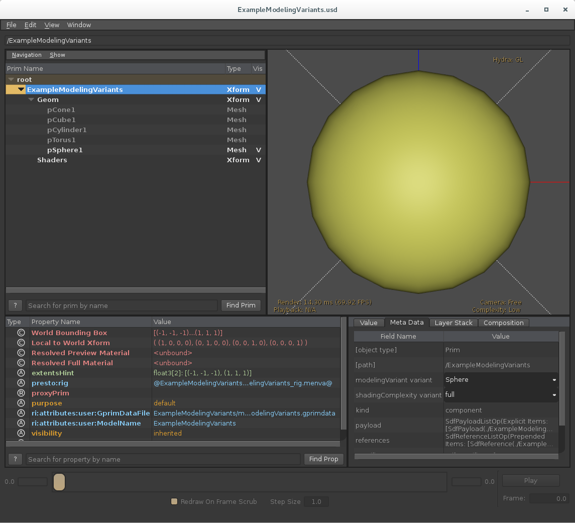

   

   From there you will see the variant change.
   从那里你会看到变量的变化。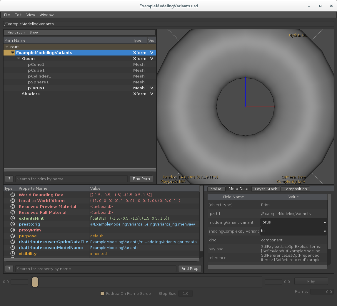

   

   Now open exampleModelingVariants.katana in Katana. The model, ExampleModelingVariants, can be toggled between its various shapes with the provided PxrUsdInVariantSelect node . Simply target the model scenegraph location and the authored variant set names will auto-populate. Select “modelingVariant” in the variantSetName parameter and the variantSelection list will populate with the shape variants.
   现在在Katana中打开exampleModelingVariants.katana。模型ExampleModelingVariants可以使用提供的PxrUsdInVariantSelect节点在其各种形状之间切换。只需定位模型场景图位置，编写的变体集名称将自动填充。在variantSetName参数中选择“modelingVariant”，variantSelection列表将填充形状变量。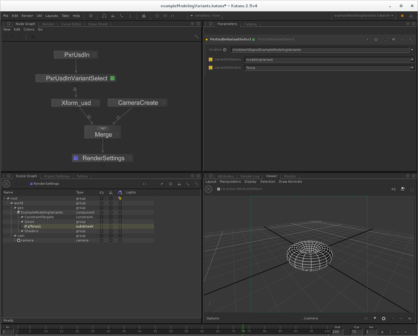

   

   Transformations, Time-sampled Animation, and Layer Offsets
   变换、时间采样动画和层偏移

   This tutorial builds an example scene of a spinning top toy that illustrates the following topics:
   本教程构建了一个旋转陀螺玩具的示例场景，其中说明了以下主题：

   We create the scene by starting with a USD file with static geometry, referencing it into another USD file, overlaying animation, and then using a third USD file to reference and re-time that animation.
   我们创建场景的方法是：从一个具有静态几何体的USD文件开始，将其引用到另一个USD文件中，覆盖动画，然后使用第三个USD文件来引用和重新计时该动画。

   To fully illustrate these concepts, we walk through a Python script that performs these steps using the Python USD API, as well as showing the resulting text .usda outputs.
   为了充分说明这些概念，我们将使用Python USD API来执行这些步骤，并显示生成的text .usda输出。

   The scripts and data files exist in the USD distribution under USD/extras/usd/tutorials/animatedTop. Run generate_examples.py in that directory to generate all of the snippets for each step shown below.
   脚本和数据文件位于USD/extras/usd/tutorials/animatedTop下的USD发行版中。在该目录中运行generate_examples.py，为下面所示的每个步骤生成所有代码片段。

   Static Geometry 静态几何体

   The toy geometry was modeled in Houdini as a revolved curve, followed by per-face color assignments as Houdini vertex attributes. The model was exported to the file USD/extras/usd/tutorials/animatedTop/top.geom.usd.
   玩具几何体在Houdini中被建模为旋转曲线，随后是作为Houdini顶点属性的每个面的颜色分配。模型被导出到文件USD/extras/usd/tutorials/animatedTop/top. geom. usd。

   The USD distribution ships with usdview, a lightweight tool for inspecting USD files. Running usdview on the file, we can see that the geometry looks like this:
   USD发行版附带了usdview，这是一个用于检查USD文件的轻量级工具。在文件上运行usdview，我们可以看到几何体看起来像这样：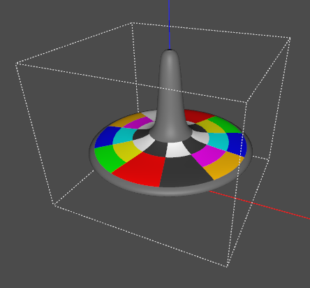

   

   Choosing an “Up” axis
   选择“向上”轴

   Computer graphics pipelines almost always pick an axis to represent the “up” direction. Common choices are +Y and +Z.
   计算机图形管线几乎总是选择一个轴来表示“向上”方向。常见的选项是+Y和+Z。

   As a pipeline interchange format, USD provides ways to configure a site default, as well as to store an explicit choice per-file. See Encoding Stage UpAxis for details.
   作为管道交换格式，USD提供了配置站点默认值以及存储每个文件的显式选择的方法。有关详细信息，请参见编码载物台上轴。

   In the examples here, we use +Z as the up axis, and write this choice out in every file so that they will work regardless of your site configuration.
   在这里的示例中，我们使用+Z作为上轴，并将此选择写入每个文件中，以便无论您的站点配置如何，它们都可以工作。

   Moving Objects with Animated Transformations: Spinning the Top
   使用动画变换移动对象：旋转顶部

   Let’s make the top spin. In a typical production pipeline, rigging & animation would be set up in a dedicated package and the results exported to USD. Here, we will create the USD files by hand to illustrate the underlying concepts.
   我们来上旋。在典型的生产流水线中，装配和动画将在专用包中设置，并将结果导出到USD。在这里，我们将手工创建USD文件来说明基本概念。

   USD represents animation as time-sampled attribute values. To establish the time range over which values are animated, the root layer can specify a start and end time in its layer metadata. We will use USD’s cinema default of 24 frames per second, and design the spinning motion to repeat after 192 frames, or 8 seconds. Setting this range up in Step1.usda:
   USD将动画表示为时间采样属性值。若要建立设置值动画的时间范围，根层可以在其层元数据中指定开始和结束时间。我们将使用USD的电影默认值24帧每秒，并将旋转运动设计为在192帧或8秒后重复。在Step1.usda中设置此范围：

   Step 1 步骤1

   # This is an example script from the USD tutorial,
   # "Transformations, Time-sampled Animation, and Layer Offsets".
   #
   # When run, it will generate a series of usda files in the current
   # directory that illustrate each of the steps in the tutorial.
   #
   from pxr import Usd, UsdGeom, Gf, Sdf
   
   def MakeInitialStage(path):
       stage = Usd.Stage.CreateNew(path)
       UsdGeom.SetStageUpAxis(stage, UsdGeom.Tokens.z)
       stage.SetStartTimeCode(1)
       stage.SetEndTimeCode(192)
       return stage
   
   def Step1():
       stage = MakeInitialStage('Step1.usda')
       stage.SetMetadata('comment', 'Step 1: Start and end time codes')
       stage.Save()
   

   Step1.usda Step1.usda

   #usda 1.0
   (
       "Step 1: Start and end time codes"
       endTimeCode = 192
       startTimeCode = 1
       upAxis = "Z"
   )
   

   You can run usdview on this file, but the viewport will be mostly empty since we haven’t added any geometry.
   你可以在这个文件上运行usdview，但是由于我们没有添加任何几何体，所以视口大部分是空的。

   Let’s add a reference to the static top model, using the UsdReferences API:
   让我们使用UsdReferences API添加对静态顶级模型的引用：

   Step 2 步骤2

   def AddReferenceToGeometry(stage, path):
       geom = UsdGeom.Xform.Define(stage, path)
       geom.GetPrim().GetReferences().AddReference('./top.geom.usd')
       return geom
   
   def Step2():
       stage = MakeInitialStage('Step2.usda')
       stage.SetMetadata('comment', 'Step 2: Geometry reference')
       top = AddReferenceToGeometry(stage, '/Top')
       stage.Save()
   

   Step2.usda Step2.usda

   #usda 1.0
   (
       "Step 2: Geometry reference"
       endTimeCode = 192
       startTimeCode = 1
       upAxis = "Z"
   )
   
   def Xform "Top" (
       prepend references = @./top.geom.usd@
   )
   {
   }
   

   This adds a Top prim to our scene, with the details referenced in from the geometry file.
   这将向我们的场景中添加一个Top prim，并从几何体文件中引用细节。

   Why prepend? 为什么要提前？

   You may have noticed the prepend operation in the reference statement above. Prepend means that, when this layer is composed with others to populate the stage, the reference will be inserted before any references that might exist in weaker sublayers. This ensures that the contents of the reference will contribute stronger opinions than any reference arcs that might exist in other, weaker layers.
   您可能已经注意到了上面引用语句中的prepend操作。Prepend意味着，当此层与其他层组合以填充阶段时，引用将插入到可能存在于较弱子层中的任何引用之前。这确保了引用的内容将比可能存在于其他较弱层中的任何引用弧贡献更强的意见。

   In other words, prepend gives the intuitive result you’d expect when you apply one layer on top of another. This is what the UsdReferences API will create by default. You can specify other options with the position parameter, but this should rarely be necessary.
   换句话说，当你在另一个层上应用一个层时，prepend会给出你所期望的直观结果。这就是UsdReferences API默认创建的内容。您可以使用position参数指定其他选项，但很少需要这样做。

   Next, let’s add animation overrides to make the top spin.
   接下来，让我们添加动画覆盖来制作上旋。

   Spatial transformations, such as rotations or translation, are a standard concept in computer graphics. USD represents transformations (also known as “xforms” for short) using the UsdGeomXformable schema. It can encode these kinds of operations as a set of related attributes. Here, we will add a spin rotation on the Z axis, and use time-samples to vary the rotation amount, in degrees:
   诸如旋转或平移的空间变换是计算机图形学中的标准概念。USD表示使用UsdGeomXformable模式的转换（也简称为“xforms”）。它可以将这些类型的操作编码为一组相关属性。在这里，我们将在Z轴上添加自旋旋转，并使用时间样本来改变旋转量（以度为单位）：

   Step 3 步骤3

   def AddSpin(top):
       spin = top.AddRotateZOp(opSuffix='spin')
       spin.Set(time=1, value=0)
       spin.Set(time=192, value=1440)
   
   def Step3():
       stage = MakeInitialStage('Step3.usda')
       stage.SetMetadata('comment', 'Step 3: Adding spin animation')
       top = AddReferenceToGeometry(stage, '/Top')
       AddSpin(top)
       stage.Save()
   

   Step3.usda Step3.usda

   #usda 1.0
   (
       "Step 3: Adding spin animation"
       endTimeCode = 192
       startTimeCode = 1
       upAxis = "Z"
   )
   
   def Xform "Top" (
       prepend references = @./top.geom.usd@
   )
   {
       float xformOp:rotateZ:spin.timeSamples = {
           1: 0,
           192: 1440,
       }
       uniform token[] xformOpOrder = ["xformOp:rotateZ:spin"]
   }
   

   UsdGeomXformable uses the name of the attribute to encode its meaning. Here, the rotateZ part specifies a rotation on the Z axis, and spin is a descriptive suffix. There are similar names for related transformation operations; see the UsdGeomXformable schema for details. Even though there is only a single transform at the moment, to make it take effect we must express the desired order as the xformOpOrder attribute.
   UsdGeomXformable使用属性的名称对其含义进行编码。这里，rotateZ部件指定Z轴上的旋转，spin是一个描述性后缀。相关的转换操作有类似的名称;有关详细信息，请参见UsdGeomXformable模式。尽管目前只有一个转换，但要使其生效，我们必须将所需的顺序表示为xformOpOrder属性。

   USD applies a linear interpolation filter to reconstruct the attribute value from the time samples. Rotations are expressed in degrees, so this provides 4 revolutions over the course of the 192-frame animation.
   USD应用线性插值滤波器从时间样本重构属性值。旋转以度表示，因此在192帧动画的过程中提供4次旋转。

   We can use usdview to play back the animation:
   我们可以使用usdview来播放动画：

   

   Chaining Multiple Transformations with xformOpOrder
   使用xformOpOrder链接多个转换

   In a real spinning top, gravity causes the top to tilt. Let’s add a “tilt” rotation to represent this. Notice that we add the tilt before the spin:
   在一个真实的的旋转陀螺中，重力使陀螺倾斜。让我们添加一个“倾斜”旋转来表示这一点。请注意，我们在旋转之前添加了倾斜：

   Step 4 步骤4

   def AddTilt(top):
       tilt = top.AddRotateXOp(opSuffix='tilt')
       tilt.Set(value=12)
   
   def Step4():
       stage = MakeInitialStage('Step4.usda')
       stage.SetMetadata('comment', 'Step 4: Adding tilt')
       top = AddReferenceToGeometry(stage, '/Top')
       AddTilt(top)
       AddSpin(top)
       stage.Save()
   

   Step 4 步骤4

   #usda 1.0
   (
       "Step 4: Adding tilt"
       endTimeCode = 192
       startTimeCode = 1
       upAxis = "Z"
   )
   
   def Xform "Top" (
       prepend references = @./top.geom.usd@
   )
   {
       float xformOp:rotateX:tilt = 12
       float xformOp:rotateZ:spin.timeSamples = {
           1: 0,
           192: 1440,
       }
       uniform token[] xformOpOrder = ["xformOp:rotateX:tilt", "xformOp:rotateZ:spin"]
   }
   

   Here is the result. The spin axis is now tilted:
   这就是结果。旋转轴现在倾斜：

   

   To illustrate the importance of transformation order, here is a variation that shows what we get if we flip the order of rotations, by swapping the two entries in the xformOpOrder:
   为了说明变换顺序的重要性，这里有一个变体，通过交换xformOpOrder中的两个条目来显示如果我们翻转旋转顺序会得到什么：

   def Step4A():
       stage = MakeInitialStage('Step4A.usda')
       stage.SetMetadata('comment', 'Step 4A: Adding spin, then tilt')
       top = AddReferenceToGeometry(stage, '/Top')
       AddSpin(top)
       AddTilt(top)
       stage.Save()
   

   ...
   uniform token[] xformOpOrder = ["xformOp:rotateZ:spin", "xformOp:rotateX:tilt"]
   ...
   

   

   Interpreting xformOpOrder
   解释xformOpOrder

   One way to think about xformOpOrder is that it describes a series of transformations to apply relative to the local coordinate frame, in order.
   考虑xformOpOrder的一种方法是，它按顺序描述了一系列相对于局部坐标系应用的转换。

   	Description 说明	xformOpOrder xformOpOrder的
   First example 第一示例	Tilt the top, then spin it on its tilted axis 倾斜顶部，然后在其倾斜轴上旋转	[“xformOp:rotateX:tilt”, “xformOp:rotateZ:spin”] [“xformOp：rotateX：tilt”，“xformOp：rotateZ：spin”]
   Second example 第二个例子	Spin the top, then tilt it in that coordinate frame 旋转顶部，然后在那个坐标系中倾斜	[“xformOp:rotateZ:spin”, “xformOp:rotateX:tilt”] [“xformOp：rotateZ：spin”，“xformOp：rotateX：tilt”]

   This suggests one more detail we’d like to add: precession. Assuming the top is sitting on a surface, torque from gravity will introduce precession, swinging the primary axis of spin around. Friction at the contact point will also cause the top to move slightly on the surface. Restoring the original xformOpOrder, we can model these effects with two more operations:
   这暗示了我们想添加的另一个细节：岁差假设陀螺位于一个表面上，来自重力的扭矩将引入进动，使旋转的主轴摆动。接触点处的摩擦也会导致顶部在表面上轻微移动。恢复原始的xformOpOrder，我们可以通过另外两个操作对这些效果进行建模：

   Step 5 步骤5

   def AddOffset(top):
       top.AddTranslateOp(opSuffix='offset').Set(value=(0, 0.1, 0))
   
   def AddPrecession(top):
       precess = top.AddRotateZOp(opSuffix='precess')
       precess.Set(time=1, value=0)
       precess.Set(time=192, value=360)
   
   def Step5():
       stage = MakeInitialStage('Step5.usda')
       stage.SetMetadata('comment', 'Step 5: Adding precession and offset')
       top = AddReferenceToGeometry(stage, '/Top')
       AddPrecession(top)
       AddOffset(top)
       AddTilt(top)
       AddSpin(top)
       stage.Save()
   

   Step5.usda Step5.usda

   #usda 1.0
   (
       "Step 5: Adding precession and offset"
       endTimeCode = 192
       startTimeCode = 1
       upAxis = "Z"
   )
   
   def Xform "Top" (
       prepend references = @./top.geom.usd@
   )
   {
       float xformOp:rotateX:tilt = 12
       float xformOp:rotateZ:precess.timeSamples = {
           1: 0,
           192: 360,
       }
       float xformOp:rotateZ:spin.timeSamples = {
           1: 0,
           192: 1440,
       }
       double3 xformOp:translate:offset = (0, 0.1, 0)
       uniform token[] xformOpOrder = ["xformOp:rotateZ:precess", "xformOp:translate:offset", "xformOp:rotateX:tilt", "xformOp:rotateZ:spin"]
   }
   

   Here is the result:
   结果如下：

   

   To summarize: we used time-samples to animate the motion, and careful ordering of the transformations to express a spinning motion with precession and translation in a relatively simple way. USD uses linear interpolation to reconstruct the intermediate values of the operations and then computes the combined transformation.
   总结如下：我们使用时间采样来使运动动画化，并且仔细地对变换进行排序，以便以相对简单的方式表达具有进动和平移的旋转运动。USD使用线性插值来重建运算的中间值，然后计算组合变换。

   Re-timing animation with Layer Offsets
   使用层偏移重新计时动画

   In the scenes above we referenced the static geometry before adding animation, but it is also possible to reference a file containing its own animation.
   在上面的场景中，我们在添加动画之前引用了静态几何体，但也可以引用包含其自身动画的文件。

   While referencing animation, a layer offset can be used to apply a simple scale & offset operation to the timeline.
   在引用动画时，层偏移可用于对时间轴应用简单的缩放和偏移操作。

   Here we reference the above animation in 3 times, adding a different +X translation to each. The first top has no layer offset; the second has a +96 frame offset (causing it to be 180 degrees out of phase), and the third top has a scale of 0.25 (causing its animation to play back at 4x the rate).
   在这里，我们将上述动画引用3次，每次添加不同的+X平移。第一顶部没有层偏移;第二个具有+96帧偏移（使其相位相差180度），第三个顶部具有0.25的比例（使其动画以4倍的速率回放）。

   Step 6 步骤6

   def Step6():
       # Use animated layer from Step5
       anim_layer_path = './Step5.usda'
   
       stage = MakeInitialStage('Step6.usda')
       stage.SetMetadata('comment', 'Step 6: Layer offsets and animation')
   
       left = UsdGeom.Xform.Define(stage, '/Left')
       left_top = UsdGeom.Xform.Define(stage, '/Left/Top')
       left_top.GetPrim().GetReferences().AddReference(
           assetPath = anim_layer_path,
           primPath = '/Top')
   
       middle = UsdGeom.Xform.Define(stage, '/Middle')
       middle.AddTranslateOp().Set(value=(2, 0, 0))
       middle_top = UsdGeom.Xform.Define(stage, '/Middle/Top')
       middle_top.GetPrim().GetReferences().AddReference(
           assetPath = anim_layer_path,
           primPath = '/Top',
           layerOffset = Sdf.LayerOffset(offset=96))
   
       right = UsdGeom.Xform.Define(stage, '/Right')
       right.AddTranslateOp().Set(value=(4, 0, 0))
       right_top = UsdGeom.Xform.Define(stage, '/Right/Top')
       right_top.GetPrim().GetReferences().AddReference(
           assetPath = anim_layer_path,
           primPath = '/Top',
           layerOffset = Sdf.LayerOffset(scale=0.25))
   
       stage.Save()
   

   Step6.usda Step6.usda

   #usda 1.0
   (
       "Step 6: Layer offsets and animation"
       endTimeCode = 192
       startTimeCode = 1
       upAxis = "Z"
   )
   
   def Xform "Left"
   {
       def Xform "Top" (
           prepend references = @./Step5.usda@</Top>
       )
       {
       }
   }
   
   def Xform "Middle"
   {
       double3 xformOp:translate = (2, 0, 0)
       uniform token[] xformOpOrder = ["xformOp:translate"]
   
       def Xform "Top" (
           prepend references = @./Step5.usda@</Top> (offset = 96)
       )
       {
       }
   }
   
   def Xform "Right"
   {
       double3 xformOp:translate = (4, 0, 0)
       uniform token[] xformOpOrder = ["xformOp:translate"]
   
       def Xform "Top" (
           prepend references = @./Step5.usda@</Top> (scale = 0.25)
       )
       {
       }
   }
   

   

   Perhaps it is a surprise that this GIF does not loop cleanly. Let’s look at the reasons. There are several things to observe here that illustrate how time samples and layer offsets work:
   也许这是一个惊喜，这个GIF不循环干净。让我们看看原因。这里有几件事要观察，说明时间采样和层偏移如何工作：

   • A layer offset (represented as SdfLayerOffset) expresses both a scale and offset that is applied to the times of the samples when bringing the data from the layer to the stage. For a given sample, ���������=���������∗�����+������.
     层偏移（表示为SdfLayerOffset）表达在将数据从层带到级时应用于样本的时间的比例和偏移两者。对于给定的样本，

   • The middle top, with the offset of +96, does not begin rotating until 96 frames after the left top (which has no offset). The reason is that USD does not extrapolate time-samples. Outside the time range covered by samples, the nearest sample value is held. In this case, it takes 96 frames until we hit the first sample and rotation begins.
     偏移为+96的中顶在左顶（无偏移）之后96帧才开始旋转。原因是USD不推断时间样本。在样本覆盖的时间范围之外，将保留最接近的样本值。在这种情况下，需要96帧，直到我们击中第一个样本并开始旋转。

   • The right top spins quickly (4x the rate) and then stops. The 0.25 scale on its reference has “shrunk down” its timeline, so it quickly plays through. After the first 48 frames (== 192 frames * 0.25), there are no further time samples, so again the values are held and rotation stops.
     右陀螺快速旋转（4倍速率），然后停止。其参考的0.25刻度已经“缩小”了其时间轴，所以它很快就发挥了作用。在前48帧（== 192帧 * 0.25）之后，没有进一步的时间样本，因此再次保持值并且旋转停止。

   • To lay out the tops in a row, we used a parent Xform prim on each, and set the translate there. If we had referenced the Top in directly and added the translate to xformOpOrder, we would be at risk of replacing (or otherwise falling out of sync with) the underlying xformOpOrder and losing its animation. By using a separate pivot we avoid this. It’s worth noting, however, that in a production pipeline most assets do not contain animated root transforms, and so this is not necessary.
     为了将顶部排成一行，我们在每个顶部上使用父Xform prim，并在那里设置平移。如果我们直接引用Top in并将translate添加到xformOpOrder，我们将面临替换（或以其他方式与之不同步）底层xformOpOrder并丢失其动画的风险。通过使用单独的枢轴，我们避免了这一点。然而，值得注意的是，在生产管道中，大多数资产不包含动画根变换，因此这是不必要的。

   • When adding the references, we had to specify the primPath. This is because we did not set the defaultPrim metadata when creating Step5.usda; if we had done that, the primPath would not be required.
     在添加引用时，我们必须指定primPath。这是因为我们在创建Step5.usda时没有设置defaultPrim元数据;如果我们这样做了，就不需要primPath了。

   To summarize, layer offsets are intended to support simple cases of retiming animation. For more elaborate scenarios, such as looping animations, USD supports the more powerful (and correspondingly more complex) concept of Value Clips.
   总而言之，层偏移旨在支持重定时动画的简单情况。对于更复杂的场景，如循环动画，USD支持更强大（相应地也更复杂）的值剪辑概念。

   We conclude this tutorial with a path-traced render of the above scene, which illustrates how the varying rates of rotation yield corresponding degrees of motion blur.
   我们以上述场景的路径跟踪渲染来结束本教程，它说明了不同的旋转速率如何产生相应程度的运动模糊。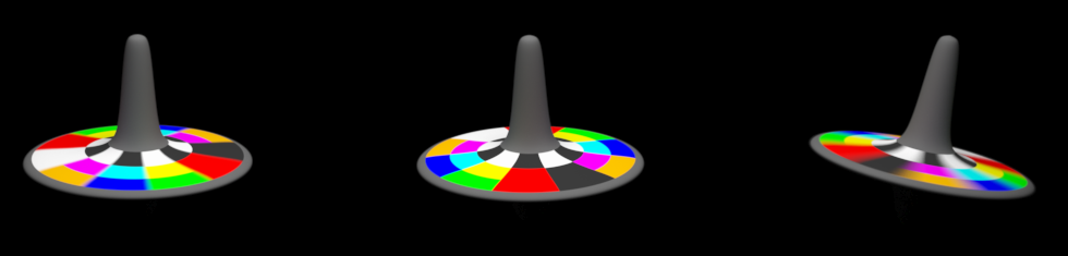

   

    

   Simple Shading in USD
   简单着色（USD）

   This tutorial demonstrates how to create a simple textured material and bind it to geometry in USD. In it we:
   本教程演示如何创建简单的纹理材质并将其绑定到USD几何体。我们在其中：

   Make a Model asset创建模型资源

   Add some simple geometry to the Model向模型添加一些简单的几何图形

   Make a Material to contain shading data制作包含着色数据的材质

   Add a surface shader to the Material将曲面着色器添加到材质

   Add texturing to the surface向曲面添加纹理

   And lastly, apply MaterialBindingAPI on the billboard prim, bind the Mesh to our Material and save the results!
   最后，在广告牌上应用MaterialBindingAPI，将网格绑定到我们的材质并保存结果！

   billboard.GetPrim().ApplyAPI(UsdShade.MaterialBindingAPI)
   UsdShade.MaterialBindingAPI(billboard).Bind(material)
   
   stage.Save()
   

   In usdview, we should now see something like:
   在usdview中，我们现在应该看到如下内容：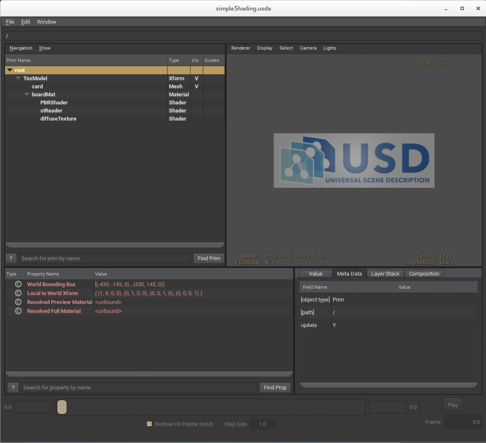

    

   

   We create the scene as a simple Model, add geometry and a Material with a simple shading network into the model, then bind the geometry to the Material.
   我们将场景创建为一个简单的模型，将几何体和具有简单着色网络的材质添加到模型中，然后将几何体绑定到材质。

   To fully illustrate these concepts, we walk through a Python script that performs the steps using the USD Python API, as well as showing the resulting text .usda outputs.
   为了充分说明这些概念，我们将介绍一个Python脚本，该脚本使用USD Python API执行这些步骤，并显示生成的text .usda输出。

   The relevant scripts and data files reside in the USD distribution in USD/extras/usd/tutorials/simpleShading. Run generate_simpleShading.py in that directory to generate all of the snippets for each step shown below.
   相关的脚本和数据文件位于USD/extras/usd/tutorials/simpleShading中。在该目录中运行generate_simpleShading.py，为下面所示的每个步骤生成所有代码段。

   Making a Model 制作模型

   The first thing we want to do is create a “container” that will hold both the geometry and the shading prims that we will create. We could have created Mesh and Material prims at root scope in the scene, but by putting them both under a common “model prim”, we make it possible to reference this asset as a whole into other scenes. In a python shell, execute the following:
   我们要做的第一件事是创建一个“容器”，它将容纳我们将要创建的几何体和着色素。我们本可以在场景中的根范围创建网格和材质prim，但是通过将它们都放在一个共同的“模型prim”下，我们可以将此资源作为一个整体引用到其他场景中。在Python shell中，执行以下操作：

   from pxr import Gf, Kind, Sdf, Usd, UsdGeom, UsdShade
   
   stage = Usd.Stage.CreateNew("simpleShading.usd")
   UsdGeom.SetStageUpAxis(stage, UsdGeom.Tokens.y)
   
   modelRoot = UsdGeom.Xform.Define(stage, "/TexModel")
   Usd.ModelAPI(modelRoot).SetKind(Kind.Tokens.component)
   

   Adding a Mesh “Billboard”
   添加网格“公告牌”

   In the interests of simplicity and brevity, we stick with a very simple piece of geometry, a quadrilateral “billboard”, with a st texture coordinate that maps the corners of the quadrilateral to the unit square in uv texture space. Note that we do not create any normals for our Mesh; this is because by default meshes use catmull-clark subdivision (to change the subdivision scheme, use UsdGeom.Mesh.CreateSubdivisionSchemeAttr()) which provide analytically computed normals to a renderer.
   为了简单和简洁，我们坚持使用一个非常简单的几何图形，一个四边形“广告牌”，它的st纹理坐标将四边形的角映射到uv纹理空间中的单位正方形。请注意，我们不创建任何法线为我们的网格;这是因为默认情况下，网格使用catmull-clark细分（要更改细分方案，请使用UsdGeom.Mesh.CreateSubdivisionSchemeAttr（）），它为渲染器提供分析计算的法线。

   billboard = UsdGeom.Mesh.Define(stage, "/TexModel/card")
   billboard.CreatePointsAttr([(-430, -145, 0), (430, -145, 0), (430, 145, 0), (-430, 145, 0)])
   billboard.CreateFaceVertexCountsAttr([4])
   billboard.CreateFaceVertexIndicesAttr([0,1,2,3])
   billboard.CreateExtentAttr([(-430, -145, 0), (430, 145, 0)])
   texCoords = UsdGeom.PrimvarsAPI(billboard).CreatePrimvar("st",
                                       Sdf.ValueTypeNames.TexCoord2fArray,
                                       UsdGeom.Tokens.varying)
   texCoords.Set([(0, 0), (1, 0), (1,1), (0, 1)])
   
   
   stage.Save()
   

   Let’s take a look at what we have so far. The last step above saved the current state of the stage into simpleShading.usd (USD files can be edited and saved multiple times). In another command shell, try:
   让我们看看目前为止我们都有什么。上面的最后一步将舞台的当前状态保存到simpleShading.usd中（USD文件可以多次编辑和保存）。在另一个命令shell中，尝试：

   > usdview simpleShading.usd
   

   We should see something like:
   我们应该看到类似这样的内容：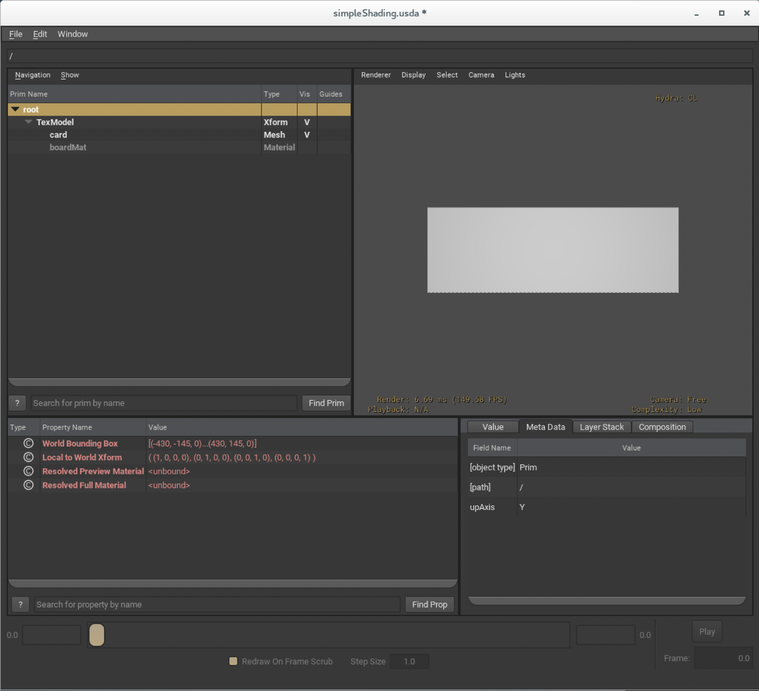

    

   

   Make a Material 制作材质

   In USD, we “bind” geometry to Material prims in order to customize how the geometry should be shaded. A Material is a container for networks of shading prims; a Material can contain one network that defines the surface illuminance response, and another that defines surface displacement . It can also contain different networks for different renderers that don’t share a common shading language. Complex models will define multiple materials, binding different geometry (Gprims) to different Materials.
   在USD中，我们将几何体“绑定”到Material prims，以自定义几何体的着色方式。材质是着色素网络的容器; a材质可以包含一个定义表面照度响应的网络和另一个定义表面位移的网络。它还可以为不同的渲染器包含不同的网络，这些渲染器不共享公共着色语言。复杂模型将定义多种材料，将不同的几何体（GPrims）绑定到不同的材料。

   In our model, we have only one gprim, and therefore need only a single Material - let us create it!
   在我们的模型中，我们只有一个gprim，因此只需要一个Material -让我们创建它！

   material = UsdShade.Material.Define(stage, '/TexModel/boardMat')
   

   Add a UsdPreviewSurface
   添加Usd预览曲面

   The most important shader in our Material will be the “surface” shader. We create it (and any other shaders in the network) as children of the material prim - this is what it means for the Material to be a container for the shading network, and is an important property to preserve. We set the surface’s metallic and roughness properties to get familiar with setting shader input properties. Any input whose value we do not set will be filled in by the renderer with the fallback value defined in the shader specification . After creating the shader, we connect the material’s surface output to the UsdPreviewSurface ‘s surface output - this is what identifies the source of the Material’s surface shading.
   材质中最重要的着色器将是“表面”着色器。我们将其（以及网络中的任何其他着色器）创建为材质prim的子级-这意味着材质将成为着色网络的容器，并且是要保留的重要属性。我们设置表面的金属和粗糙度属性，以熟悉设置着色器输入属性。任何未设置值的输入将由渲染器使用着色器规范中定义的回退值填充。创建着色器后，我们将材质的表面输出连接到UsdPreviewSurface的表面输出-这是标识材质表面着色源的内容。

   pbrShader = UsdShade.Shader.Define(stage, '/TexModel/boardMat/PBRShader')
   pbrShader.CreateIdAttr("UsdPreviewSurface")
   pbrShader.CreateInput("roughness", Sdf.ValueTypeNames.Float).Set(0.4)
   pbrShader.CreateInput("metallic", Sdf.ValueTypeNames.Float).Set(0.0)
   
   material.CreateSurfaceOutput().ConnectToSource(pbrShader.ConnectableAPI(), "surface")
   

   Add Texturing 添加纹理

   The last step is to add a texture as the source for the surface’s diffuseColor . Texturing requires two nodes in the shading network: aUsdUVTexturenode to read and map the texture, and a UsdPrimvarReader (more precisely, aUsdPrimvarReader_float2, the implementation that reads float2Array-valued Primvar s) to fetch a texture coordinate from each piece of geometry bound to the material, to inform the texture node how to map surface coordinates to texture coordinates.
   最后一步是添加一个纹理作为表面的diffuseColor的源。纹理需要着色网络中的两个节点：aUsdUVTexture节点用于读取和映射纹理，以及UsdPrimvarReader（更准确地说，aUsdPrimvarReader_float2，读取float 2Array-valuePrimvar s的实现）用于从绑定到材质的每个几何体中获取纹理坐标，以通知纹理节点如何将表面坐标映射到纹理坐标。

   stReader = UsdShade.Shader.Define(stage, '/TexModel/boardMat/stReader')
   stReader.CreateIdAttr('UsdPrimvarReader_float2')
   
   diffuseTextureSampler = UsdShade.Shader.Define(stage,'/TexModel/boardMat/diffuseTexture')
   diffuseTextureSampler.CreateIdAttr('UsdUVTexture')
   diffuseTextureSampler.CreateInput('file', Sdf.ValueTypeNames.Asset).Set("USDLogoLrg.png")
   diffuseTextureSampler.CreateInput("st", Sdf.ValueTypeNames.Float2).ConnectToSource(stReader.ConnectableAPI(), 'result')
   diffuseTextureSampler.CreateOutput('rgb', Sdf.ValueTypeNames.Float3)
   pbrShader.CreateInput("diffuseColor", Sdf.ValueTypeNames.Color3f).ConnectToSource(diffuseTextureSampler.ConnectableAPI(), 'rgb')
   

   Note that we have not yet specified what texture coordinate (primvar) the PrimvarReader should read. We could author the name of the primvar directly on its varname input. However, we instead demonstrate how we can connect shader inputs to “public interface attributes” on Materials. Any input in a shading network can connect to an input on its enclosing material, and the renderer will migrate the Material input’s authored value (if any) to any shader input connected to it before rendering and shading begins. In effect, this gives us a way to “expose” inputs deep in a shading network for easy overriding by consumers of the Material, since all the inputs on a Material will be exposed and editable without needing to look inside the Material, which may contain many shading prims.
   请注意，我们还没有指定PrimvarReader应该读取的纹理坐标（primvar）。我们可以直接在primvar的varname输入上编写primvar的名称。但是，我们将演示如何将着色器输入连接到材质上的“公共接口属性”。着色网络中的任何输入都可以连接到其封闭材质上的输入，并且渲染器将在渲染和着色开始之前将“材质”输入的编写值（如果有）迁移到与其连接的任何着色器输入。实际上，这为我们提供了一种在着色网络深处“暴露”输入的方法，以便材质的消费者轻松覆盖，因为材质上的所有输入都将被暴露和可编辑，而无需查看材质内部，其中可能包含许多着色素。

   stInput = material.CreateInput('frame:stPrimvarName', Sdf.ValueTypeNames.Token)
   stInput.Set('st')
   
   stReader.CreateInput('varname',Sdf.ValueTypeNames.Token).ConnectToSource(stInput)
   

   
   You can now try viewing this:
   你现在可以试试看这个：

   usdview models/Ball/Ball.usd
   # in usdview, you can view the different levels of subdivision via ctrl+- and ctrl+=
   

   Exporting the table asset
   导出表资源

   Open the Table.ma file in Maya.
   在Maya中打开Table.ma文件。

   maya assets/Table/Table.ma
   

   Select the table in the scene, then select File ‣ Export Selection. Choose pxrUsdExport under Files of type .
   选择场景中的表格，然后选择“文件”“导出当前选择”。在“文件类型”下选择“pxrUsdExport”。

   As with the Ball, be sure to choose RfM under shading mode . In the file browser, find models/Table/Table.maya.usd and save over it.
   与球一样，确保在着色模式下选择RfM。在文件浏览器中，找到models/Table/Table.maya.usd并将其保存。

   At this point, you should have geometry and shading information authored for both the Ball and Table. If you were not able to complete this section, see the note above for instructions on copying over pre-exported assets.
   此时，您应该为球和桌编写了几何体和着色信息。如果您无法完成此部分，请参阅上面的注释，了解有关复制预导出资源的说明。

   Shading Variants 着色变体

   We will add shading variants to the Ball entirely through code. Please see tutorial_scripts/add_shadingVariants.py.
   我们将完全通过代码向球添加着色变体。请参见tutorial_scripts/add_shadingVariants.py。

   Start by copying the Ball textures into your Ball directory:
   首先将“Ball”纹理复制到“Ball”目录中：

   cp -r assets/Ball/tex models/Ball/
   

   Add shading variants to the Ball with a python script:
   使用python脚本为球添加着色变体：

   python tutorial_scripts/add_shadingVariants.py
   
   usdcat models/Ball/Ball.shadingVariants.usda
   

   This script assumes you’ve been following along the tutorial and is expecting a Ball model to exist with shading from the Maya file. If you’ve tweaked things, you may have to go in and modify that script.
   此脚本假定您一直在沿着教程，并且期望存在具有Maya文件中的着色的Ball模型。如果您已经调整了一些东西，那么您可能必须进入并修改该脚本。

   We are keeping the networks very simple for this tutorial. If you look at the Ball model in usdview, and then with :filename`/Ball` selected, select the Meta Data tab and use the shadingVariant drop-down menu to change to variants with different colors.
   在本教程中，我们保持网络非常简单。如果您在usdview中查看Ball模型，然后选择：filename`/Ball`，选择Meta Data选项卡并使用shadingVariant下拉菜单更改为不同颜色的变体。

   usdview models/Ball/Ball.usd
   

   

   Set dressing 套装敷料

   We’ll create a set model that brings together the Table and a standard set of 15 Ball models together.
   我们将创建一个集合模型，将Table和一组标准的15个Ball模型组合在一起。

   python tutorial_scripts/create_Room_set.py
   usdview models/Room_set/Room_set.usd
   

   This script assumes you’ve been following along the tutorial and is expecting a Ball and Table model to exist. It also makes some assumptions about the size of these models. If you’ve tweaked things, you may have to go in and modify that script.
   此脚本假定您已经沿着教程进行了操作，并且期望存在球和桌子模型。它还对这些模型的大小做了一些假设。如果您已经调整了一些东西，那么您可能必须进入并修改该脚本。

   Also, note that we’re hard-coding absolute paths to the other assets. The path resolver plugin provides a better mechanism that allows you to locate assets by other means.
   另外，请注意，我们硬编码了到其他资产的绝对路径。路径解析器插件提供了一种更好的机制，允许您通过其他方式定位资产。

   You may need to move the camera around to see the table and balls as pictured below.
   您可能需要移动相机来查看桌子和球，如下图所示。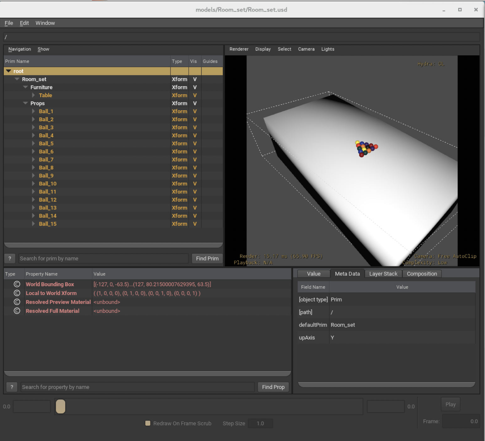

   

   Shot Work 喷丸作业

   Here, we’ll mock up an example of how a sequence and shot might be structured. This will illustrate some of the benefits of USD composition. Since your structure likely varies, we’ll first define some terms and explain the structure we’re about to create.
   在这里，我们将模拟一个如何构建序列和镜头的示例。这将说明USD组合的一些好处。由于您的结构可能会有所不同，我们将首先定义一些术语并解释我们将要创建的结构。

   A sequence is a collection of related shots. A shot will include (by sublayering) all the scene description that is associated with its sequence. This structure allows you to put opinions that affect multiple shots in one location. We will also make each sequence inherit opinions from a global/shared shot.usd file. This makes it so we can define the overall structure in one place. That’s a good place to put things you will need everywhere (for example, the camera).
   序列是相关快照的集合。快照将包括（通过子层）与其序列相关联的所有场景描述。此结构允许您将影响多个快照的意见放在一个位置。我们还将使每个序列从全局/共享的shot.usd文件中继承意见。这使得我们可以在一个地方定义整体结构。这是一个很好的地方，把你需要的东西（例如，相机）。

   Another axis by which we organize our work is by department. A shot can have a layer for layout, a layer for animation, and a layer for sim, as an example. The same goes for a sequence. We will build a shot that has the following layers (strongest to weakest)
   我们组织工作的另一个轴心是部门。作为示例，镜头可以具有用于布局的层、用于动画的层和用于sim的层。序列也是如此。我们将建立一个镜头，有以下几层（最强到最弱）

   # shot layers
   s00_01.usd
   s00_01_sim.usd
   s00_01_anim.usd
   s00_01_layout.usd
   s00_01_sets.usd
   
   # sequence layers
   s00.usd
   s00_sim.usd
   s00_anim.usd
   s00_layout.usd
   s00_sets.usd
   
   # global
   shot.usd
   

   Note 注记

   USD has no notion of what a “shot” or “sequence” is. Again, this is just an example and this structure is not required for USD.
   USD没有“镜头”或“序列”的概念。同样，这只是一个示例，USD不需要此结构。

   Sequence/Shot setup 序列/镜头设置

   The scripts/create_shot.py script will help setup a sequence and a shot. For starters, take a look at the structure that’s defined in assets/shot.usd:
   scripts/create_shot.py脚本将帮助设置序列和快照。对于初学者，请看一下assets/shot.usd中定义的结构：

   usdcat assets/shot.usd
   

   Let’s setup the sequence. We’ll use the create_shot.py script even though we’re making a sequence:
   我们来设定一下顺序。我们将使用create_shot.py脚本，即使我们正在制作一个序列：

   python scripts/create_shot.py s00 -o shots/s00 -b assets/shot.usd
   

   This creates a sequence in the directory shots/s00 that references assets/shot.usd (note the -b argument to create_shot.py authors that reference verbatim).
   这将在shots/s 00目录中创建一个序列，该序列引用assets/shot.usd（注意create_shot.py作者的参数是逐字引用的）。

   And now the shot:
   现在镜头：

   python scripts/create_shot.py s00_01 -o shots/s00_01 -b shots/s00/s00.usd
   

   Now, you should have the layer structure defined in the previous sections. Opinions from the shot will override the weaker opinions that are in the sequence or the “global” layer.
   现在，您应该已经拥有了前面几节中定义的层结构。来自镜头的意见将覆盖序列或“全局”层中较弱的意见。

   Note 注记

   In an actual production, you’ll probably structure your files to make the dependency between s00_01 and s00 more evident.
   在实际的生产环境中，您可能会对文件进行结构化，以使s00_01和s 00之间的依赖性更加明显。

   Since this is a newly created shot and sequence, there shouldn’t really be anything in it except for what was in assets/shot.usd, which should just be the camera.
   由于这是一个新创建的快照和序列，除了assets/shot.usd中的内容之外，其中不应该有任何内容，而assets/shot.usd中的内容应该只是相机。

   usdview shots/s00_01/s00_01.usd
   

   Simple shot work 简单的拍摄工作

   Now we’ll start running some scripts. First, at the sequence level, we’ll bring in the Room_set asset.
   现在我们将开始运行一些脚本。首先，在序列级别，我们将引入Room_set资产。

   python tutorial_scripts/add_set_to_s00.py
   usdview shots/s00/s00.usd
   

   And now, let’s say a layout TD adds in a cue ball, removes some un-needed props, and positions the camera
   现在，让我们说一个布局TD添加了一个母球，删除一些不需要的道具，并定位相机

   # notice that s00_01 brings in opinions from s00
   usdview shots/s00_01/s00_01.usd
   
   # feel free to introspect the resulting files in between each of the following.
   python tutorial_scripts/layout_shot_s00_01.py
   python tutorial_scripts/anim_shot_s00_01.py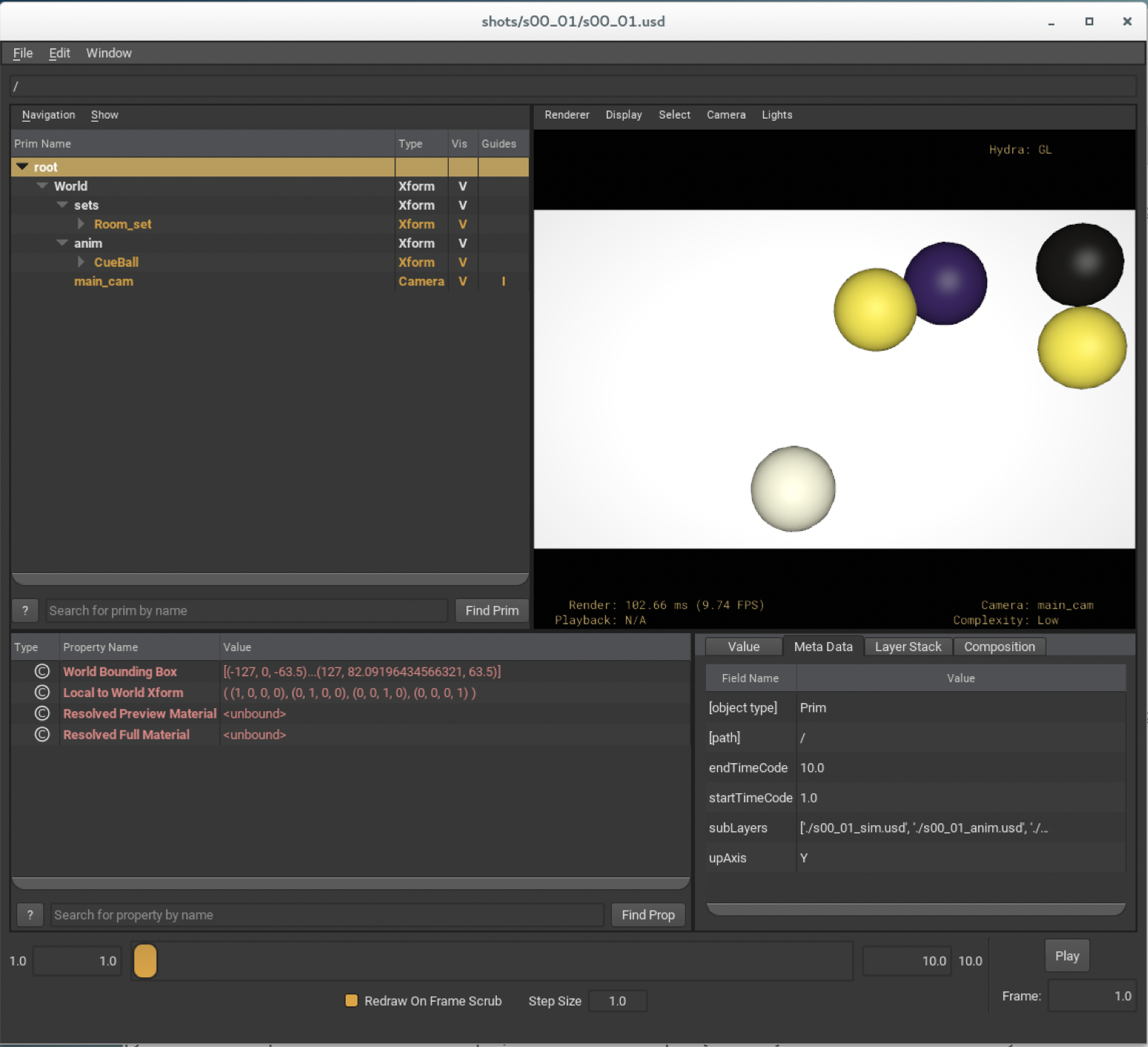
   

   

   Render Render 

   Note 注记

   The Katana USD plugin was removed from the USD distribution in version 20.05 in favor of the Foundry-supported plugin hosted on GitHub. This portion of the tutorial is not regularly tested but remains for historical reference.
   Katana USD插件在20.05版本中从USD发行版中删除，以支持托管在GitHub上的Foundry支持的插件。本教程的这一部分不定期测试，但仍作为历史参考。

   We’ll now render our shot in Katana. In the root of your endToEnd tutorial directory, run:
   我们现在用武士刀来渲染镜头。在endToEnd教程目录的根目录中，运行：

   katana assets/simple.katana
   

   The USD file is read in with the provided PxrusdIn node. An optional camera is merged into the scene (to work around a known issue when rendering from the camera in the USD file). A simple light is created in the gaffer node.
   使用提供的PxrusdIn节点读入USD文件。将可选摄影机合并到场景中（以解决从USD文件中的摄影机渲染时的已知问题）。在gaffer节点中创建一个简单的灯光。

   To render the scene, right-click on the RenderSettings node and select “Preview Render”.
   要渲染场景，请右键单击“RenderSettings”节点，然后选择“预览渲染”。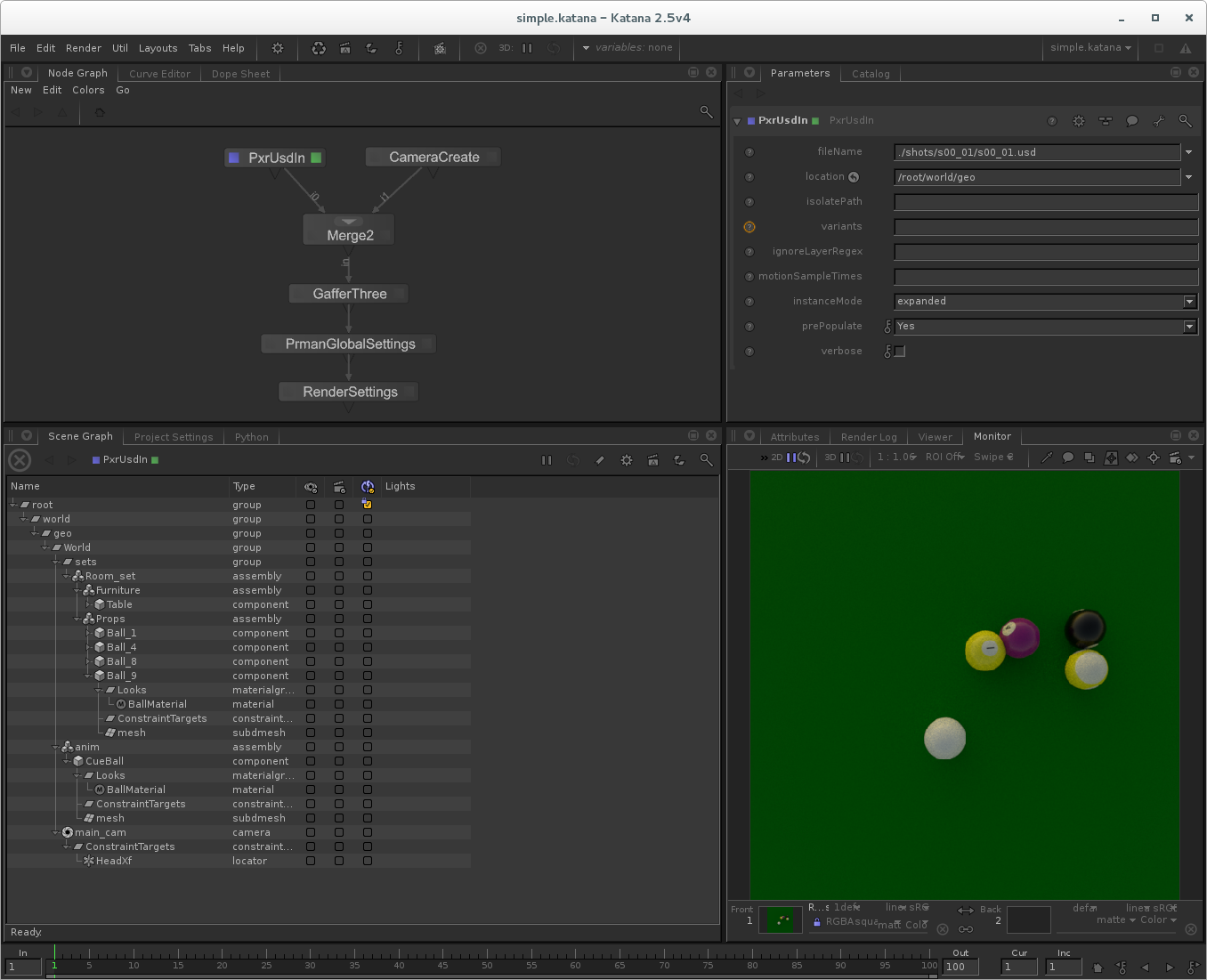

   

   That’s it! 就是这样！

   Feel free to experiment with this tutorial by modifying scripts or adding your own geometry and shading.

    

   Houdini USD Example Workflow
   Houdini USD示例工作流程

   Note 注记

   The Houdini USD plugin was removed from the USD distribution in version 20.05 in favor of native USD support in Houdini Solaris. This documentation remains for historical reference.
   Houdini USD插件在20.05版本中从USD发行版中删除，以支持Houdini Solaris中的原生USD支持。本文件仅供参考。

   An example of using Houdini in a USD-centric pipeline
   在以美元为中心的管道中使用Houdini的示例

   Authoring USD Overrides in Houdini
   在Houdini中创作USD Overrides

   This tutorial shows an example using Houdini to modify the transform of model in a USD scene. The files for this tutorial live in USD/extras/usd/tutorials/Houdini. It is assumed that you have a working knowledge of Houdini.
   本教程展示了一个使用Houdini修改USD场景中模型变换的示例。本教程的文件位于USD/extras/usd/tutorials/Houdini。假设你有霍迪尼的工作知识。

   In summary you will do the following:
   总之，您将执行以下操作：

   1. View the USD Scene - use usdview to determine what you need to import into Houdini.
      查看USD场景-使用usdview来确定您需要导入到Houdini中的内容。

   2. Import the USD geometry - import all the geometry to modify and anything needed for reference into Houdini.
      导入美元几何-导入所有的几何修改和任何需要参考到胡迪尼。

   3. Houdini Shot work - modifying the imported models position, orientation et al.
      Houdini拍摄工作-修改导入模型的位置，方向等。

   4. Export the chages to a USD Overlay.
      将更改导出到USD叠加。

   5. Insert the Overlay back into the USD Scene.
      将叠加插入到USD场景中。

   View the USD Scene
   查看USD场景

   Open the USD scene in usdview to identify the geometry you want to modify by using the following command line.
   使用以下命令行在usdview中打开USD场景，以标识要修改的几何体。

   $ usdview  USD/extras/usd/tutorials/Houdini/shot.usda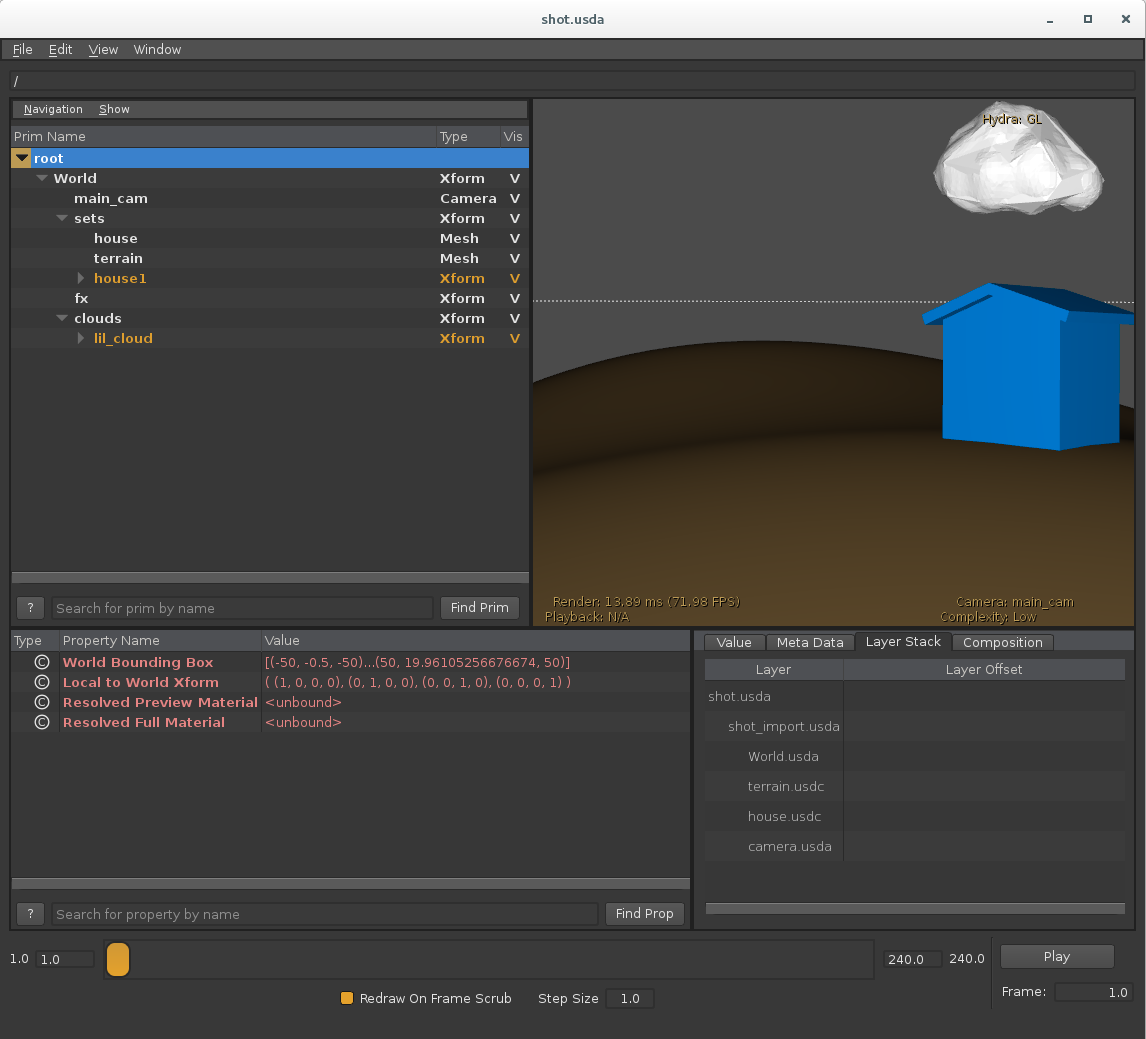
   

   

   In this case we are interested in the little red house at the origin:
   在这种情况下，我们感兴趣的是原点的小红房子：

   • First select the prim by clicking in the prim browser on the ‘house’ row.
     首先通过点击prim浏览器中的'house'行来选择prim。

   • Next hit ‘f’ to bring it into frame.
     下一个点击'f'将其带入帧中。

   

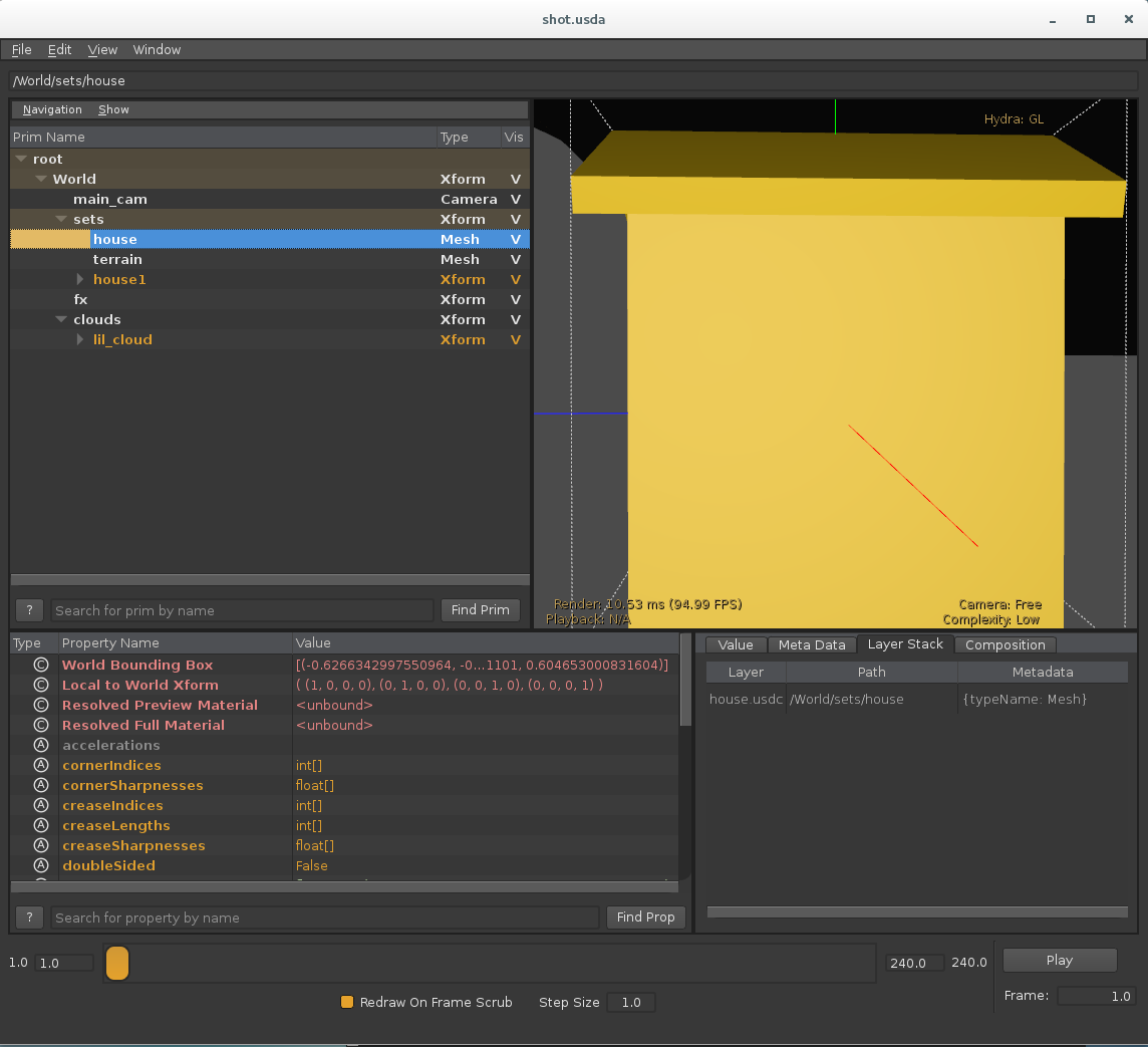
   Note 注记

   Note that the house appears yellow because we have selected it.
   请注意，房子显示为黄色，因为我们已经选择了它。

   You can find the name of the prim path of the house in this USD stage(/World/sets/house) by looking at the Prim Name window in the upper left hand corner of usdview. You’ll use this information later when we import the house into Houdini.
   您可以通过查看usdview左手角的Prim Name窗口来找到此USD阶段中房屋的prim路径名称（/World/sets/house）。稍后将房子导入Houdini时，您将使用此信息。

   Imagine that you have received a note that the house should be placed at the top of the highest hill on the terrain.
   想象一下，你已经收到了一张纸条，房子应该放在地形上最高的山顶上。

   Import USD geometry into Houdini
   将USD几何图形导入Houdini

   It’s time to import the little red house into Houdini.
   是时候把小红屋导入胡迪尼了。

   1. From the Geometry context in Houdini drop down a USD import SOP.
      从Houdini中的几何上下文下拉一个USD导入SOP。

   2. Enter the name of, or browse to the USD file that contains the stage you’re interested in modifying in the “USD File” parameter, in this case: USD/extras/usd/tutorials/Houdini/shot.usda
      在“USD文件”参数中输入包含您要修改的阶段的USD文件的名称，或浏览到该文件，在本例中：USD/extras/usd/tutorials/Houdini/shot.usda

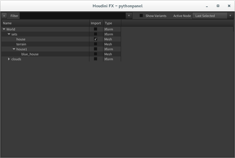
   3. Enter the name of USD Prim path you are interested in modifying into the “Prim Path” parameter, in this case: /World/sets/house. You can also use the Tree view to visually browse through the USD stage to select the prim path.
      在“Prim Path”参数中输入您要修改的USD Prim路径的名称，在本例中：/World/sets/house.您还可以使用树视图来直观地浏览USD阶段以选择prim路径。

   

   In this case we also need to set the “Traversal” parameter to Gprims
   在本例中，我们还需要将“Traversal”参数设置为GPrims

   The above steps sets set the traversal criteria for importing geometry into Houdini
   上述步骤集设置了将几何体导入Houdini的遍历条件

   You should now see the little red house in your Houdini viewport.
   现在，您应该在Houdini视口中看到小红屋。

   On middle mouse click of the usdimport SOP you will notice that there is one primitive, a packed USD. As you will only be altering the transformation of this model you can keep it packed and export what is known as a transform overlay.
   鼠标中键点击usdimport SOP时，您会注意到有一个原语，即打包的USD。由于您将只更改此模型的变换，因此可以将其打包并导出所谓的变换叠加。

   Import the terrain for visual reference.
   导入地形以供视觉参考。

   Repeat the steps above to import the terrain model by duplicating the usdimport SOP and replacing the “Prim Path” with /World/sets/terrain and templating the new usdimport SOP.
   重复上述步骤，通过复制usdimport SOP并将“Prim Path”替换为/World/sets/terrain并模板化新的usdimport SOP来导入地形模型。

   Houdini shot work 胡迪尼射击工作

   Use the transform sop to move the house to the top of the highest hill.
   使用变换SOP将房子移到最高的山顶。

   Export the USD Overlay
   导出美元覆盖图

   1. Create a “USD Output” ROP in the Outputs context of Houdini.
      在Houdini的Outputs上下文中创建一个“USD Output”ROP。

   2. Enter the path to the transform sop you used to move the little red house.
      输入路径的转换SOP你用来移动小红房子。

   3. Toggle the “Overlay Existing Geometry” Parameter on.
      打开“覆盖现有几何图形”参数。

   4. Enter the path of the new USD file that will contain the overlay, in this case: USD/extras/usd/tutorials/Houdini/OVR_house.usda
      输入将包含覆盖的新USD文件的路径，在本例中：USD/extras/usd/tutorials/Houdini/OVR_house.usda

   5. Enter the file path of the USD file that contains the USD prim you wish to override into the “Overlay Reference File” parameter, in this case: USD/extras/usd/tutorials/Houdini/shot.usda
      在“Overlay Reference File”参数中输入包含要覆盖的USD prim的USD文件的文件路径，在本例中：USD/extras/usd/tutorials/Houdini/shot.usda

   6. As you are only interested in altering the transform of our model we are going to uncheck “Overlay All” and check “Overlay Transforms”.
      由于你只对改变模型的变换感兴趣，我们将取消选中“覆盖所有”并选中“覆盖变换”。

   

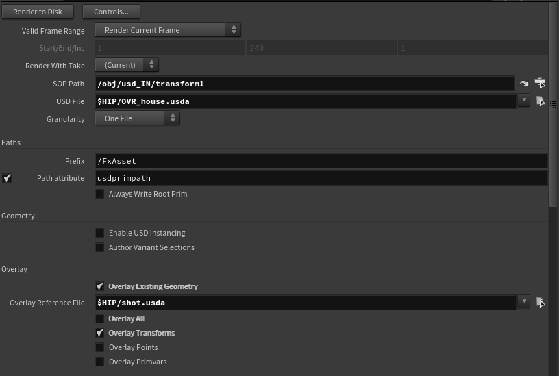
   Hit “Render to Disk”
   点击“渲染到磁盘”

   Insert Overlay into USD Scene
   将叠加插入USD场景

   1. Drop down a “USD Layer” ROP into the Outputs context of Houdini.
      将“USD层”ROP下拉到Houdini的Outputs上下文中。

   2. Set the first “Source” paramter field to USD/extras/usd/tutorials/Houdini/OVR_house.usda
      将第一个“Source”参数字段设置为USD/extras/usd/tutorials/Houdini/OVR_house.usda

   3. Hit “Render to Disk” on the USD layer ROP.
      点击USD层ROP上的“渲染到磁盘”。

   If everything has gone according to plan, you should now be able to see the house in it’s new location at the top of the hill in usdview:
   如果一切都按计划进行，您现在应该可以在usdview中看到位于山顶的新位置的房子：

   The completed Houdin file can be found here: USD/extras/usd/tutorials/Houdini/overlay_tutorial.hip
   完整的Houdin文件可以在这里找到：USD/extras/usd/tutorials/Houdini/overlay_tutorial.hip

   You can see other example of how to use USD in Houdini in the included hip file: USD/extras/usd/tutorials/Houdini/examples.hip
   您可以在包含的髋关节文件中看到如何在Houdini中使用USD的其他示例：USD/extras/usd/tutorials/Houdini/examples.hip