【Python机器学习】线性模型——用于二分类的线性模型

线性模型也广泛用于分类问题，对于二分类问题，可以用以下公式进行预测：

y=w[0]*x[0]+w[1]*x[1]+…………+w[p]*x[p]+b>0

公式与现行回归的公式非常类似，但没有返回特征的加权求和，而是为预测设置了阈值。如果函数值小于0，就预测类别-1，否则预测类别+1。

对于用于回归的线性模型，输出y是特征的线性函数，是直线、平面或者超平面。对于用于分类的线性模型，决策边界是输入的线性函数。

学习线性模型有很多算法，主要区别在于：

1、系数与截距的特定组合对训练数据拟合好坏的度量方法

2、是否使用正则化，以及使用哪种正则化。

最常见的线性分类算法是Logistic回归和线性支持向量机（线性SVM），用到的类分别是linear_model.LogisticRegression、svm.LinearSVC。

对两种分类算法的模型用在forge数据集上，并对决策边界可视化：

import mglearn.datasets
from sklearn.linear_model import Ridge,LinearRegression,Lasso,LogisticRegression
from sklearn.svm import LinearSVC
import matplotlib.pyplot as plt


plt.rcParams['font.sans-serif']=['SimHei']

X,y=mglearn.datasets.make_forge()

fig,axes=plt.subplots(1,2,figsize=(10,3))
for model,ax in zip([LinearSVC(),LogisticRegression()],axes):
    clf=model.fit(X,y)
    mglearn.plots.plot_2d_separator(clf,X,fill=False,eps=0.5,ax=ax,alpha=.7)
    mglearn.discrete_scatter(X[:,0],X[:,1],y,ax=ax)
    ax.set_title('{}'.format(clf.__class__.__name__))
    ax.set_xlabel('0')
    ax.set_ylabel('1')
axes[0].legend()
plt.show()

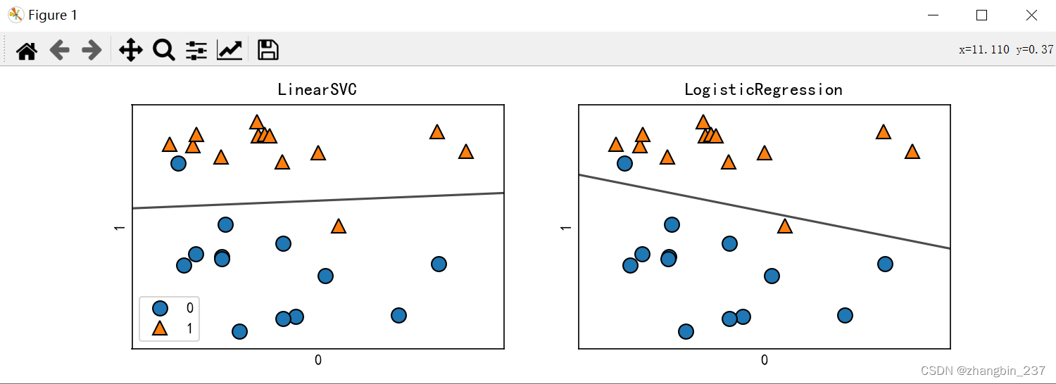
图中黑线上方的数据点会被划分为类别1，下方的数据点会被划分为类别0。

两种模型默认使用L2正则化，就像岭回归。 

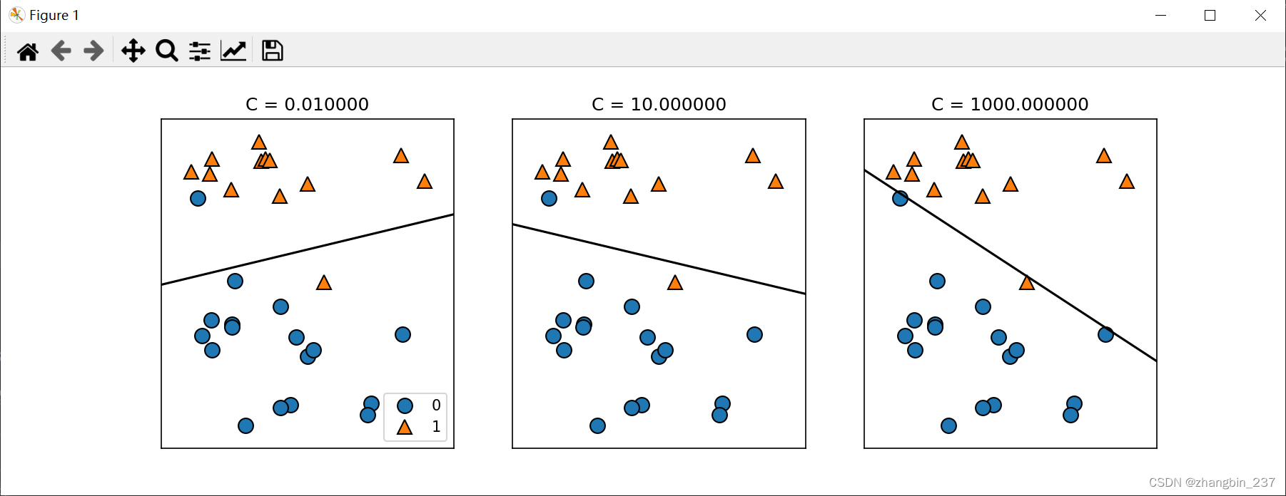
对于LogisticRegression和LinearSVC，决定正则化强度的权衡参数为C，C越大，正则化越弱，也就是C越小，训练集拟合越好，C越大，系数向量越接近于0。

对于多维数据集，用于分类的线性模型会非常强大，考虑更多特征时，避免过拟合就更重要。

from sklearn.datasets import load_breast_cancer
from sklearn.model_selection import train_test_split
from sklearn.linear_model import Ridge,LinearRegression,Lasso,LogisticRegression


cancer=load_breast_cancer()
X_train,X_test,y_train,y_test=train_test_split(
    cancer.data,cancer.target,stratify=cancer.target,random_state=42
)
logreg=LogisticRegression().fit(X_train,y_train)
print('C=1的训练集score:{:.3f}'.format(logreg.score(X_train,y_train)))
print('C=1的测试集score:{:.3f}'.format(logreg.score(X_test,y_test)))


logreg_100=LogisticRegression(C=100).fit(X_train,y_train)
print('C=100的训练集score:{:.3f}'.format(logreg_100.score(X_train,y_train)))
print('C=100的测试集score:{:.3f}'.format(logreg_100.score(X_test,y_test)))


logreg_001=LogisticRegression(C=0.01).fit(X_train,y_train)
print('C=0.01的训练集score:{:.3f}'.format(logreg_001.score(X_train,y_train)))
print('C=0.01的测试集score:{:.3f}'.format(logreg_001.score(X_test,y_test)))

结果输出：

C=1的训练集score:0.944
C=1的测试集score:0.965
C=100的训练集score:0.955
C=100的测试集score:0.958
C=0.01的训练集score:0.934
C=0.01的测试集score:0.930

 可以看到，C=1（默认值）时，性能就比较好了，训练集和测试集的精度在95%左右，但非常相近，所以模型很可能是欠拟合的，C=100时，得到了更高的训练集精度，C=0.01时精度下降，有可能存在过拟合。

对于系数的影响，可视化可以看到：

from sklearn.datasets import load_breast_cancer
from sklearn.model_selection import train_test_split
from sklearn.linear_model import Ridge,LinearRegression,Lasso,LogisticRegression
import matplotlib.pyplot as plt


plt.rcParams['font.sans-serif']=['SimHei']
cancer=load_breast_cancer()
X_train,X_test,y_train,y_test=train_test_split(
    cancer.data,cancer.target,stratify=cancer.target,random_state=42
)
logreg=LogisticRegression().fit(X_train,y_train)
logreg_100=LogisticRegression(C=100).fit(X_train,y_train)
logreg_001=LogisticRegression(C=0.01).fit(X_train,y_train)
#,penalty ='l1',solver='liblinear'
plt.plot(logreg.coef_.T,'s',label='logreg C=1')
plt.plot(logreg_100.coef_.T,'^',label='logreg C=100')
plt.plot(logreg_001.coef_.T,'v',label='logreg C=0.01')
plt.xticks(range(cancer.data.shape[1]),cancer.feature_names,rotation=90)
plt.hlines(0,0,cancer.data.shape[1])
plt.ylim(-5,5)
plt.xlabel('index')
plt.ylabel('系数大小')
plt.legend()
plt.show()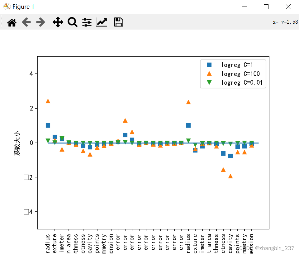

 

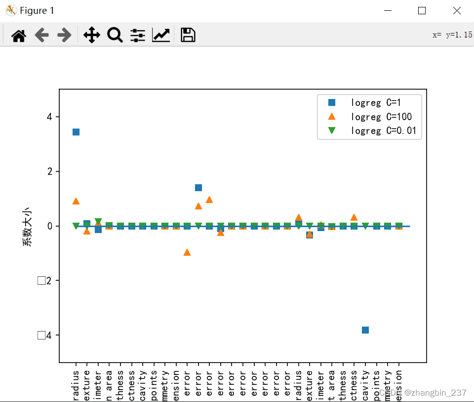
可以看到，更强的正则化使得系数更倾向于0，但不正好等于0，如果用L1正则化，约束模型就只使用少数几个特征，