python 拟牛顿法 求非线性方程_不动点法和牛顿法求解非线性方程的数值解（Python）...

首发公众号：120701101.

---

一、不动点法

1、代码

# -*- coding: utf-8 -*-
"""
Created on Tue Jun 30 17:01:54 2020

@author: 120701101
@Email: 18********30@163.com

"""

# 导入相关计算库
import numpy as np
import matplotlib
import matplotlib.pyplot as plt
# 设置LaTex字体样式
from matplotlib import rcParams
config = {
    "font.family":'serif',
    "font.size": 25,
    "mathtext.fontset":'stix',
    "font.serif": ['SimSun'],
}
rcParams.update(config)


# --------------------------------fixedPoint

def fixedPoint(g, x1, stepmax, tol):
    ## g是由y=y(x)转化来的
    
    x = np.zeros(stepmax)
    x[1] = x1
    
    for n in range(1, stepmax+1):
        
        x[n+1] = g(x[n])
        
        if abs(x[n+1] - x[n]) < tol: return x[n+1]
        
        
# 求解过程                
g = lambda x: 2 ** (-x)
x_real = fixedPoint(g, 0, stepmax = 25, tol = 1.0e-6)
print("x_real = ", "{:7.6f}".format(x_real))      


# 绘制结果
plt.figure(figsize=(10,5), dpi=300)
x = np.linspace(0, 1.6, 500)
plt.plot(x,g(x), '-k', linewidth=2, label=r"$g = 2^{-x}$")
plt.plot([x[-1], x[0]], [x[-1], x[0]], linestyle="-.", color="grey")
plt.plot(x_real, g(x_real), 'o-r', markersize=15, label=r"$(0, g(0))$")

plt.xlabel(r"$x$")
plt.ylabel(r"$y(x)$")
plt.title("不动点法求解非线性函数的根", fontsize=20)
plt.xlim((0, 1.6))
plt.xticks(np.arange(0, 1.7, 0.2))
plt.legend()
plt.grid(True, linestyle='-.')
plt.annotate("这是" + r"$x=2^{-x}$" + "的解", xy=(x_real, g(x_real)),
             xytext=(x_real-0.1, g(x_real)+0.35),
             arrowprops=dict(arrowstyle="->",connectionstyle="arc3,rad=.2"))

plt.show()

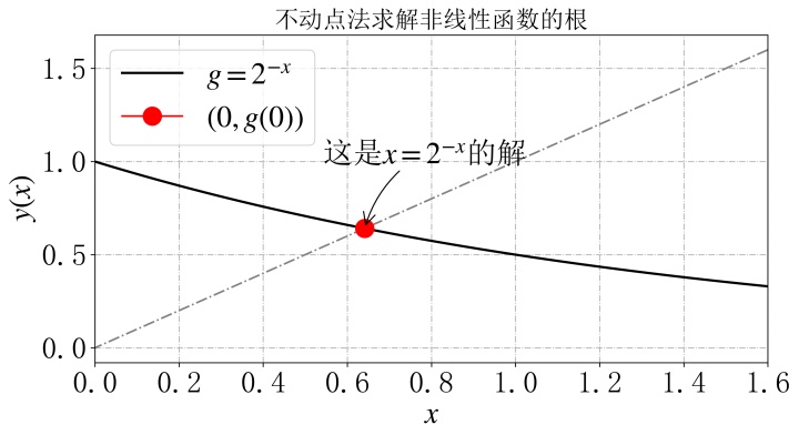
2、计算结果

运行代码即可得到，

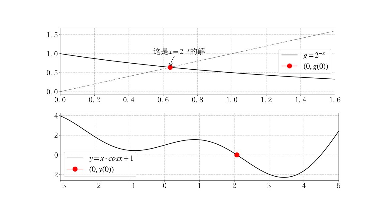
x_real =  0.641186

3、图像结果

不动点法

二、牛顿法

1、代码

# -*- coding: utf-8 -*-
"""
Created on Tue Jun 30 18:12:53 2020

@author: 120701101
@Email: 18********30@163.com

"""

import numpy as np
from numpy import sign
import matplotlib
import matplotlib.pyplot as plt

from matplotlib import rcParams

config = {
    "font.family":'serif',
    "font.size": 25,
    "mathtext.fontset":'stix',
    "font.serif": ['SimSun'],
}
rcParams.update(config)

# ----------------------------newton

def newton(fun, df, x1, stepmax, tol):
    ## df是原方程的导数方程
    x = np.zeros(stepmax+1)
    x[1] = x1
    
    for k in range(1, stepmax+1):
        
        if sign(df(x[k])) == 0: return print("请重新输入正确的初始值")
        
        x[k+1] = x[k] - fun(x[k]) / df(x[k])
        
        if abs(x[k+1] - x[k]) < tol: return x[k+1]
        
        
# 求解过程                
fun = lambda x: x * np.cos(x) + 1
df = lambda x: np.cos(x) - x * np.sin(x)
x_real = newton(fun, df, 1, stepmax = 25, tol = 1.0e-6)
print("x_real = ", "{:7.6f}".format(x_real))
            

# 绘制结果
plt.figure(figsize=(10,5), dpi=300)
x = np.linspace(-3, 5, 500)
plt.plot(x,fun(x), '-k', linewidth=2, label=r"$y = x cdot cosx + 1$")
plt.plot(x_real, fun(x_real), 'o-r', markersize=15, label=r"$(0, y(0))$")

plt.xlabel(r"$x$")
plt.ylabel(r"$y(x)$")
plt.title("牛顿法求解非线性函数的根", fontsize=20)
plt.xlim((-3, 5))
plt.xticks(np.arange(-3, 6, 1))
plt.legend()
plt.grid(True, linestyle='-.')

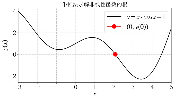
plt.show()

2、计算结果

运行代码即可得到，

x_real =  2.073933

3、图像结果

牛顿法

三、简评

python写的牛顿法不如matlab的方便，python写的需要自己先求出原非线性方程的导数方程，没有像matlab的matlabFunction符号函数转化为句柄函数的函数功能。