PyTorch中的18种损失函数使用教程

---

1. 损失函数（Loss Function）：衡量模型输出与真实值之间的差异。
   $$Loss=f(y,\hat{y})$$

2. 代价函数（Cost Function）：
   $$Cost=\frac{1}{N}\sum _{i=1}^{N}f(y_i,{\hat{y}}_i)$$

3. 目标函数（(Objective Function）：
   $$Obj=Cost+Regularization$$
   目标函数以最小化 $Cost$ 为目标，同时为了避免过拟合，还需要添加正则项 $Regularization$，常用的正则化方法，包括 L1正则化（稀疏正则化）和 L2正则化（权重衰减正则化）。

---

1. CrossEntropyLoss()

交叉熵损失函数适用于分类任务。官方文档：LINK

torch.nn.CrossEntropyLoss(weight: Optional[torch.Tensor] = None, 
                          size_average=None, 
                          ignore_index: int = -100, 
                          reduce=None, 
                          reduction: str = 'mean')

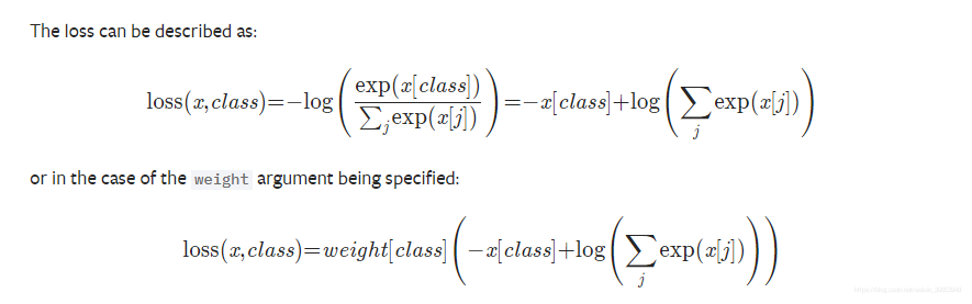
功能：结合 nn.LogSoftmax 与 nn.NLLLoss，计算交叉熵。

• 这一函数并非公式意义上的交叉熵函数计算，它采用softmax()将数据归一化到概率输出区间。因为交叉熵函数常用于分类任务，分类任务通常需要计算两个输出的概率值。交叉熵衡量两个概率分布之间的差异。交叉熵值越低，两个分布越相似。

参数说明：

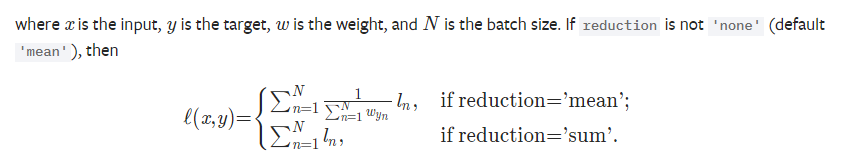
• weight：分类权重设置；各类别的loss的权重。
• size_average：已弃用
• reduce：已弃用
• ignore_index：忽略某个类别的索引；
• reduction：计算模式选择；包括：none-逐个元素计算；sum-所有元素求和，返回标量；mean-加权平均，返回标量。

---

计算公式：

---

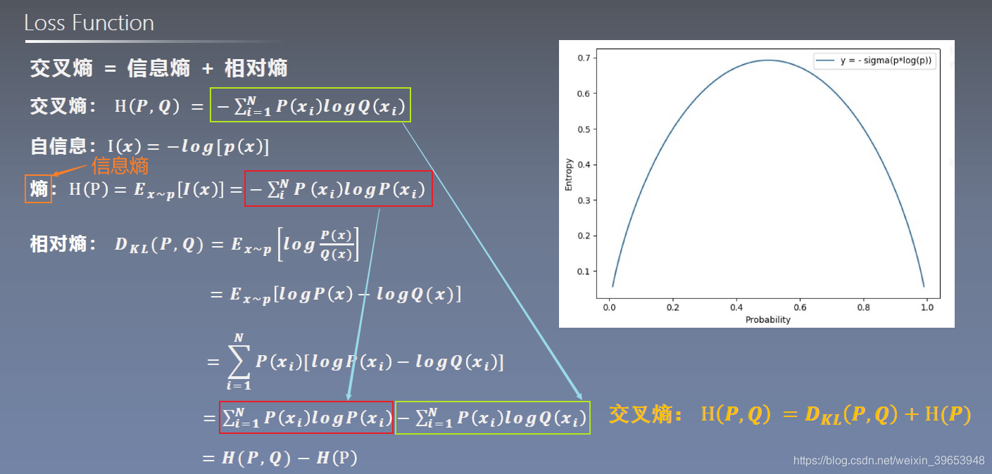
• 熵（entropy）：在信息论中，熵是接收的每条消息中包含的信息的平均量，又被称为信息熵、信源熵、平均自信息量。这里，“消息”代表来自分布或数据流中的事件、样本或特征。（熵最好理解为不确定性的量度而不是确定性的量度，因为越随机的信源的熵越大。）来自信源的另一个特征是样本的概率分布。1948年，克劳德·艾尔伍德·香农将热力学的熵，引入到信息论，因此它又被称为香农熵(Shannon entropy)。
• 熵的概念最早起源于物理学，用于度量一个热力学系统的无序程度。在信息论里面，熵是对不确定性的测量。但是在信息世界，熵越高，则能传输越多的信息，熵越低，则意味着传输的信息越少。
• KL散度（Kullback-Leibler divergence，KLD），在讯息系统中称为相对熵（relative entropy），在连续时间序列中称为随机性（randomness），在统计模型推断中称为讯息增益（information gain）。也称讯息散度（information divergence）。
• KL散度是两个概率分布P和Q差别的非对称性的度量。 KL散度是用来度量使用基于Q的分布来编码服从P的分布的样本所需的额外的平均比特数。典型情况下，P表示数据的真实分布，Q表示数据的理论分布、估计的模型分布、或P的近似分布。
• 在信息论中，自信息（self-information），由克劳德·香农提出，是与概率空间中的单一事件或离散随机变量的值相关的信息量的量度。自信息的期望值就是信息论中的熵，它反映了随机变量采样时的平均不确定程度。
• 由定义，当信息被拥有它的实体传递给接收它的实体时，仅当接收实体不知道信息的先验知识时信息才得到传递。如果接收实体事先知道了消息的内容，这条消息所传递的信息量就是0。只有当接收实体对消息对先验知识少于100%时，消息才真正传递信息。因此，一个随机产生的事件 ${\omega }_n$ 所包含的自信息数量，只与事件发生的几率相关。事件发生的几率越低，在事件真的发生时，接收到的信息中，包含的自信息越大。
• 在概率论和信息论中，两个随机变量的 互信息（mutual Information，MI） 或转移信息（transinformation）是变量间相互依赖性的量度。不同于相关系数，互信息并不局限于实值随机变量，它更加一般且决定着联合分布 p(X,Y) 和分解的边缘分布的乘积 p(X)p(Y) 的相似程度。互信息是点间互信息（PMI）的期望值。互信息最常用的单位是bit。

---

$P$ 表示数据的真实分布，$Q$ 表示估计的模型分布或 $P$ 的近似分布，由于训练集是固定，$P$ 的信息熵 $H(P)$ 是常数，在优化时常数可忽略，因此，机器学习模型中优化交叉熵等价于优化相对熵。

上图中表示伯努利两点分布非信息熵，当事件的概率=0.5时，信息熵最大（=0.69），此时不确定性最大，模型不具备任何判别能力。

---

1.1 CEL中不同计算模式的影响

import torch
import torch.nn as nn
import torch.nn.functional as F
import numpy as np

# 构造三个样本数据
inputs = torch.tensor([[1, 2], [1, 3], [1, 3]], dtype=torch.float)
# 三个样本的标签分别为第0类，第1类，第1类
target = torch.tensor([0, 1, 1], dtype=torch.long)

# CrossEntropy loss: reduction 

# def loss function
loss_f_none = nn.CrossEntropyLoss(weight=None, reduction='none')
loss_f_sum = nn.CrossEntropyLoss(weight=None, reduction='sum')
loss_f_mean = nn.CrossEntropyLoss(weight=None, reduction='mean')

# forward
loss_none = loss_f_none(inputs, target)
loss_sum = loss_f_sum(inputs, target)
loss_mean = loss_f_mean(inputs, target)

# view
print(loss_none, loss_sum, loss_mean)
'''
tensor([1.3133, 0.1269, 0.1269]) tensor(1.5671) tensor(0.5224)
'''

手动计算验证：

# 第一个样本的索引
idx = 0

# 取出第一个样本
input_1 = inputs.detach().numpy()[idx]      # [1, 2]
target_1 = target.numpy()[idx]              # [0]

# 第一项
x_class = input_1[target_1]

# 第二项
sigma_exp_x = np.sum(list(map(np.exp, input_1)))
log_sigma_exp_x = np.log(sigma_exp_x)

# 输出第一个样本对应的 loss
loss_1 = -x_class + log_sigma_exp_x

print(loss_1)
'''
1.3132617
'''

---

1.2 CEL中分类权重 weights 的影响

# def loss function
# 设置第0类的权重为1，设置第1类的权重为2
weights = torch.tensor([1, 2], dtype=torch.float)

# weights = torch.tensor([0.7, 0.3], dtype=torch.float)

loss_f_none_w = nn.CrossEntropyLoss(weight=weights, reduction='none')
loss_f_sum = nn.CrossEntropyLoss(weight=weights, reduction='sum')
loss_f_mean = nn.CrossEntropyLoss(weight=weights, reduction='mean')

# forward
loss_none_w = loss_f_none_w(inputs, target)
loss_sum = loss_f_sum(inputs, target)
loss_mean = loss_f_mean(inputs, target)

print("\nweights: ", weights)
print(loss_none_w, loss_sum, loss_mean)

输出：

weights:  tensor([1., 2.])
tensor([1.3133, 0.2539, 0.2539]) tensor(1.8210) tensor(0.3642)

说明：

• 在计算loss时，第二类的的损失乘以权重2；
• 在第三种计算模式 'mean' 下，其计算方式为加权平均，即 (1.3133+ 0.2539+0.2539)/(1+2+2)=0.3642。

---

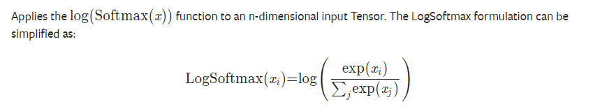
1.3 nn.LogSoftmax()

官方文档：LINK

torch.nn.LogSoftmax(dim: Optional[int] = None)

实例：

m = torch.nn.LogSoftmax()
input = torch.randn(2, 3)
output = m(input)
print(input,'\n',output)

'''
tensor([[ 2.4068, -1.1458, -0.1125],
        [-1.3691,  1.1176, -0.2194]]) 
 tensor([[-0.1036, -3.6562, -2.6229],
        [-2.7837, -0.2970, -1.6340]])
'''

---

2. nn.NLLLoss()

The negative log likelihood loss.官方文档：LINK

torch.nn.NLLLoss(weight: Optional[torch.Tensor] = None, 
                 size_average=None, 
                 reduce=None, 
                 ignore_index: int = -100, 
                 reduction: str = 'mean')

功能：实现负对数似然函数中的负号功能。

实例：

weights = torch.tensor([1, 1], dtype=torch.float)

loss_f_none_w = nn.NLLLoss(weight=weights, reduction='none')
loss_f_sum = nn.NLLLoss(weight=weights, reduction='sum')
loss_f_mean = nn.NLLLoss(weight=weights, reduction='mean')

# forward
loss_none_w = loss_f_none_w(inputs, target)
loss_sum = loss_f_sum(inputs, target)
loss_mean = loss_f_mean(inputs, target)

print("weights: ", weights)
print("NLL Loss", loss_none_w, loss_sum, loss_mean)

'''
weights:  tensor([1., 1.])
NLL Loss tensor([-1., -3., -3.]) tensor(-7.) tensor(-2.3333)
'''

---

3. nn.BCELoss()

二分类交叉熵损失函数（Binary Cross Entropy），求 inputs 和 target 之间的交叉熵。官方文档：LINK

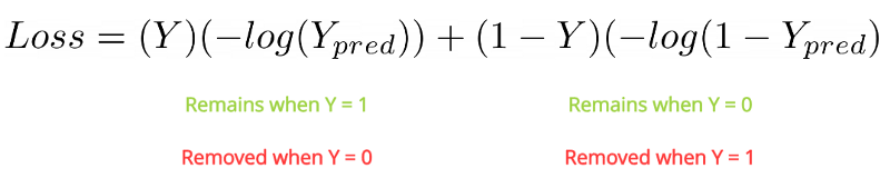
• 输入输出取值在[0,1]范围内；

代码：

# 构造样本数据
inputs = torch.tensor([[1, 2], [2, 2], [3, 4], [4, 5]], dtype=torch.float)
# 对于分类问题，分类标签需要设置成哑变量（one-hot）形式
target = torch.tensor([[1, 0], [1, 0], [0, 1], [0, 1]], dtype=torch.float)

target_bce = target

# itarget，激活之后，使得loss的输入变换到[0,1]区间内，不激活，使用BCELoss会报错
inputs = torch.sigmoid(inputs)

weights = torch.tensor([1, 1], dtype=torch.float)

loss_f_none_w = nn.BCELoss(weight=weights, reduction='none')
loss_f_sum = nn.BCELoss(weight=weights, reduction='sum')
loss_f_mean = nn.BCELoss(weight=weights, reduction='mean')

# forward
loss_none_w = loss_f_none_w(inputs, target_bce)
loss_sum = loss_f_sum(inputs, target_bce)
loss_mean = loss_f_mean(inputs, target_bce)

print("\nweights:", weights, '\n')
print("BCE Loss:\n", loss_none_w, loss_sum, loss_mean)

'''
weights: tensor([1., 1.]) 

BCE Loss:
 tensor([[0.3133, 2.1269],
        [0.1269, 2.1269],
        [3.0486, 0.0181],
        [4.0181, 0.0067]]) tensor(11.7856) tensor(1.4732)
'''

• 可以看出计算了8个Loss，每个样本有2个神经元，4个样本共8个神经元。每个神经元一一对应计算Loss。

---

4. nn.BCEWithLogitsLoss()

官方文档：LINK。

torch.nn.BCEWithLogitsLoss(weight: Optional[torch.Tensor] = None, 
                           reduction: str = 'mean', 
                           pos_weight: Optional[torch.Tensor] = None)

该函数自动结合了sigmoid函数和二分类交叉熵函数（BCELoss）。

关键参数：

• pos_weight：表示正样本的权值，该参数用来平衡正负样本，计算正样本的Loss时会乘以该系数。

inputs = torch.tensor([[1, 2], [2, 2], [3, 4], [4, 5]], dtype=torch.float)
target = torch.tensor([[1, 0], [1, 0], [0, 1], [0, 1]], dtype=torch.float)

target_bce = target

# 无需再加激活函数sigmoid
# inputs = torch.sigmoid(inputs)

weights = torch.tensor([1, 1], dtype=torch.float)
# pos_weights 参数影响
# pos_w = torch.tensor([3], dtype=torch.float)        # 3

loss_f_none_w = nn.BCEWithLogitsLoss(weight=weights, reduction='none', pos_weight=None)
loss_f_sum = nn.BCEWithLogitsLoss(weight=weights, reduction='sum', pos_weight=None)
loss_f_mean = nn.BCEWithLogitsLoss(weight=weights, reduction='mean', pos_weight=None)

# forward
loss_none_w = loss_f_none_w(inputs, target_bce)
loss_sum = loss_f_sum(inputs, target_bce)
loss_mean = loss_f_mean(inputs, target_bce)

print("\nweights:", weights, '\n')
print(loss_none_w, loss_sum, loss_mean)

'''
weights: tensor([1., 1.]) 

tensor([[0.3133, 2.1269],
        [0.1269, 2.1269],
        [3.0486, 0.0181],
        [4.0181, 0.0067]]) tensor(11.7856) tensor(1.4732)
'''

---

5. nn.L1LOSS （MAE）

mean absolute error (MAE) ，官方文档：LINK。

torch.nn.L1Loss(reduction: str = 'mean')

• 计算模型输入inputs与真实标签target之差的绝对值。
• $L_n=|x_n-y_n|$

---

6. nn.MSELoss

mean squared error (squared L2 norm)，官方文档：LINK。

torch.nn.MSELoss(reduction: str = 'mean')

• 计算模型输入inputs与真实标签target之差的平方。
• $L_n=(x_n-y_n{)}^2$

---

7. nn.SmoothL1Loss

官方文档：LINK

torch.nn.SmoothL1Loss(reduction: str = 'mean')

• $\text{loss}(x,y)=\frac{1}{n}{\sum }_i{z}_i$

• $z_i=\{\begin{array}{ll}0.5(x_i-y_i{)}^2,& \text{if }|x_i-y_i|<1\\ |x_i-y_i|-0.5,& \text{otherwise }\end{array}$

---

SmoothL1Loss 与 L1Loss 对比。

import matplotlib.pyplot as plt

# 构建 inputs，在[-3,3]上取500个数据点
inputs = torch.linspace(-3, 3, steps=500)
# 构建与 inputs 同维度的标签target，元素为0
target = torch.zeros_like(inputs)
# 一一对应求解 loss
loss_f = nn.SmoothL1Loss(reduction='none')

loss_smooth = loss_f(inputs, target)

loss_l1 = np.abs(inputs.numpy())

plt.figure(dpi=300)
plt.plot(inputs.numpy(), loss_smooth.numpy(), label='Smooth L1 Loss')
plt.plot(inputs.numpy(), loss_l1, label='L1 loss')
plt.xlabel('$x_i - y_i$')
plt.ylabel('loss value')
plt.legend(loc='best')
plt.grid()
plt.show()

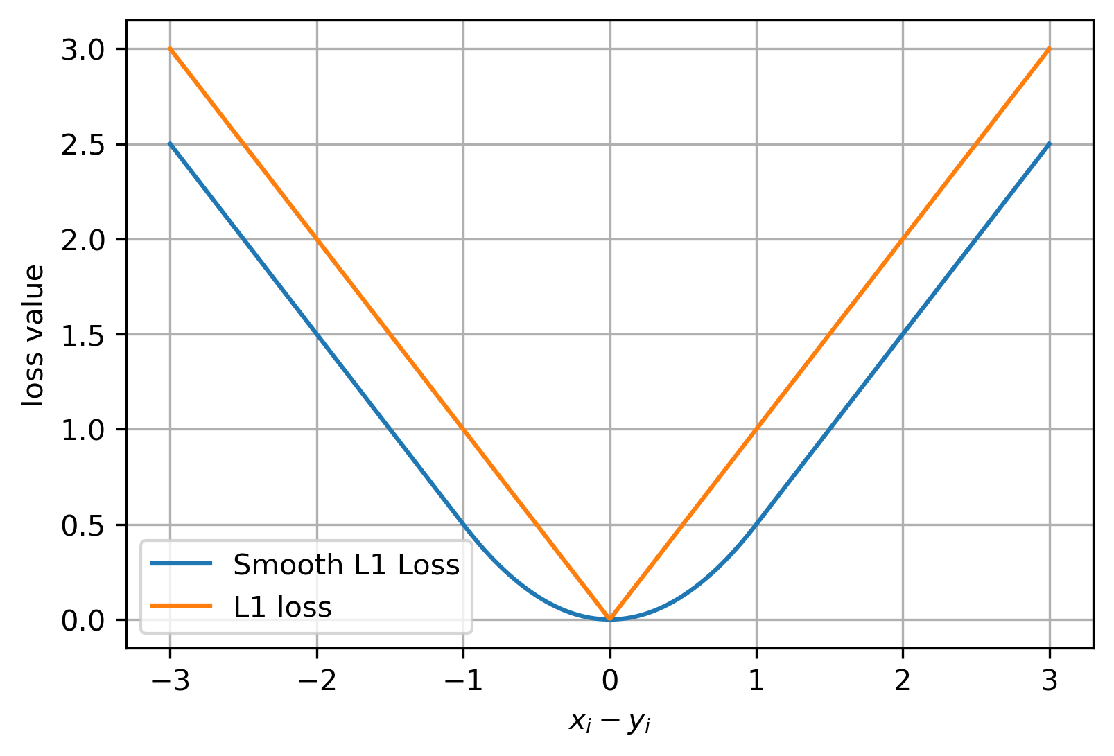
• 平滑之后，可以减轻离群点对模型的影响。

---

8. nn.PoissonNLLLoss

泊松分布的负对数似然损失函数（Negative log likelihood loss with Poisson distribution），官方文档：LINK。

torch.nn.PoissonNLLLoss(log_input: bool = True, 
                        full: bool = False, 
                        eps: float = 1e-08, 
                        reduction: str = 'mean')

• $\text{target}\sim \mathrm{Poisson}(\text{input})\text{loss}(\text{input},\text{target})=\text{input}-\text{target}\ast \log (\text{input})+\log (\text{target!})$

参数说明：

• log_input：输入是否为对数形式；if True the loss is computed as 【$\exp (\text{input})-\text{target}\ast \text{input}$】， if False the loss is $【\text{input}-\text{target}\ast \log (\text{input}+\text{eps})】$；
• full：计算所有Loss，默认为False；
• eps：修正项，避免当参数 log_input = False 时，计算 log(input)=nan，eps 默认为 1e-8。

---

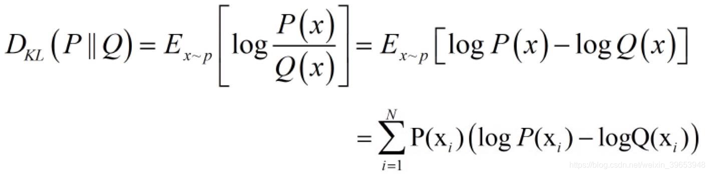
9. nn.KLDivLoss

相对熵损失函数，又称KL散度损失函数（The Kullback-Leibler divergence Loss），官方文档：LINK。

torch.nn.KLDivLoss(reduction: str = 'mean', 
                   log_target: bool = False)

参数说明：

• reduction：可选 none，sum，mean，batchmean（以batch size维度求平均值）。

由于相对熵损失函数衡量的是两个概率分布之间的差异，用来计算两个概率分布的距离。因此，应当保证输入应当在概率区间，Pytorch的KLDivLoss直接取输入计算，因而该函数会提前计算log-probabilities，通过nn.logsoftmax()实现。

---

10. nn.MarginRankingLoss

官方文档：LINK。

torch.nn.MultiLabelMarginLoss(margin: float = 0.0, reduction: str = 'mean')

• $\text{loss}(x,y)=\max (0,-y\ast (x1-x2)+\text{margin})$

功能：计算两个向量之间的相似度，用于排序任务。该方法计算两组数据之间的差异，返回1个n*n的Loss矩阵。其中 $y$ 是标签取值，只能是 $1,-1$，$x_1$、$x_2$ 是这两组向量的一个元素，计算各元素差值；margin为边界，默认为0，因此margin暂时可以忽略不考虑。$y=1$ 时，希望 $x_1>x_2$；$y=-1$时，希望 $x_1<x_2$；因此，通过计算这两种情况都不产生loss。

参数说明：

• margin：边界值，x1与x2之间的差异值；
• reduction：计算模式，none/sum/mean。

代码说明：

x1 = torch.tensor([[1], [2], [3]], dtype=torch.float)
x2 = torch.tensor([[2], [2], [2]], dtype=torch.float)

target = torch.tensor([1, 1, -1], dtype=torch.float)

loss_f_none = nn.MarginRankingLoss(margin=0, reduction='none')

loss = loss_f_none(x1, x2, target)

print(loss)

输出：

tensor([[1., 1., 0.],
        [0., 0., 0.],
        [0., 0., 1.]])

以上计算结果为：$x_1$ 的三个元素分别与 $x_2$ 的三个元素计算 loss 求得。如果数据的shape为 (n,n) ，则最后的loss矩阵也为同样的shape。

---

11. nn.MultilabelMarginLoss

多标签边界损失函数，官方文档：LINK。

torch.nn.MultiLabelMarginLoss(reduction: str = 'mean')

$$\text{loss}(x,y)=\sum _{ij}\frac{\max (0,1-(x[y[j]]-x[i]))}{\text{x.size}(0)}$$
w h e r e   x ∈ { 0 ,    ⋯   ,    x.size ( 0 ) − 1 } ,   y ∈ { 0 ,    ⋯   ,    y.size ( 0 ) − 1 } ,   0 ≤ y [ j ] ≤ x.size ( 0 ) − 1 ,   a n d i ≠ y [ j ]   f o r   a l l   i   a n d   j where \ x \in \left\{0, \; \cdots , \; \text{x.size}(0) - 1\right\}, \ y \in \left\{0, \; \cdots , \; \text{y.size}(0) - 1\right\}, \ 0 \leq y[j] \leq \text{x.size}(0)-1, \ and i \neq y[j] \ for \ all \ i \ and \ j where x∈{0,⋯,x.size(0)−1}, y∈{0,⋯,y.size(0)−1}, 0≤y[j]≤x.size(0)−1, andi=y[j] for all i and j

---

12. nn.SoftMarginLoss

计算二分类的logistic损失，官方文档：LINK。

torch.nn.SoftMarginLoss(reduction: str = 'mean')

$$\text{loss}(x,y)=\sum _i\frac{\log (1+\exp (-y[i]\ast x[i]))}{\text{x.nelement}()}$$

---

13. nn.MultiLabelSoftMarginLoss

SoftMarginLoss的多标签版本，官方文档：LINK。

torch.nn.MultiLabelSoftMarginLoss(weight: Optional[torch.Tensor] = None, 
                                  size_average=None, 
                                  reduce=None, 
                                  reduction: str = 'mean')

$loss(x,y)=-\frac{1}{C}\ast {\sum }_{i}y[i]\ast \log ((1+\exp (-x[i]){)}^{-1})+(1-y[i])\ast \log \left(\frac{\exp (-x[i])}{(1+\exp (-x[i]))}\right)$

w h e r e   i ∈ { 0 ,    ⋯   ,    x.nElement ( ) − 1 } ， ‘ y [ i ] ∈ { 0 ,    1 } where \ i \in \left\{0, \; \cdots , \; \text{x.nElement}() - 1\right\}，`y[i] \in \left\{0, \; 1\right\} where i∈{0,⋯,x.nElement()−1}，‘y[i]∈{0,1}

---

14. nn.MultiMarginLoss

计算多分类的折页损失，官方文档：LINK。

torch.nn.MultiMarginLoss(p: int = 1, 
                         margin: float = 1.0, 
                         weight: Optional[torch.Tensor] = None, 
                         reduction: str = 'mean')

参数说明：

• p：可选1或2；
• weight：各类别的loss设置权值；
• margin：边界值。

$$\text{loss}(x,y)=\frac{{\sum }_i\max (0,w[y]\ast (\text{margin}-x[y]+x[i]){)}^p)}{\text{x.size}(0)}$$

---

15. nn.TripletMarginLoss

计算三元组损失，常用于人脸验证算法，官方文档：LINK

torch.nn.TripletMarginLoss(margin: float = 1.0, 
                           p: float = 2.0, 
                           eps: float = 1e-06, 
                           swap: bool = False, 
                           reduction: str = 'mean')

• L ( a , p , n ) = max ⁡ { d ( a i , p i ) − d ( a i , n i ) + m a r g i n , 0 } L(a, p, n) = \max \{d(a_i, p_i) - d(a_i, n_i) + {\rm margin}, 0\} L(a,p,n)=max{d(ai​,pi​)−d(ai​,ni​)+margin,0}
• $d(x_i,y_i)={\Vert {\mathbf{x}}_i-{\mathbf{y}}_i\Vert }_p$

参数说明：

• p：范数的阶，默认为2。

---

16. nn.HingeEmbeddingLoss

计算两个输入的相似性，常用于非线性嵌入学习（embedding）和半监督学习。官方文档：LINK

torch.nn.HingeEmbeddingLoss(margin: float = 1.0, reduction: str = 'mean')

l n = { x n , if    y n = 1 , max ⁡ { 0 , Δ − x n } , if    y n = − 1 , l_n = \begin{cases} x_n, & \text{if}\; y_n = 1,\\ \max \{0, \Delta - x_n\}, & \text{if}\; y_n = -1, \end{cases} ln​={xn​,max{0,Δ−xn​},​ifyn​=1,ifyn​=−1,​

---

17. nn.CosineEmbeddingLoss

采用余弦相似度计算两个输入的相似性，官方文档：LINK。

$\text{loss}(x,y)=\{\begin{array}{ll}1-\cos (x_1,x_2),& \text{if }y=1\\ \max (0,\cos (x_1,x_2)-\text{margin}),& \text{if }y=-1\end{array}$

参数说明：

• margin：边界值，可取值[-1,1]，推荐[0,0.5]。
• reduction：计算模式 none，sum，mean。

---

18. nn.CTCLoss

计算CTC损失（The Connectionist Temporal Classification loss），适用于时间序列数据分类任务。官方文档：LINK。

torch.nn.CTCLoss(blank: int = 0,
                 reduction: str = 'mean', 
                 zero_infinity: bool = False)

参数说明：

• blank：blank label；
• zero_infinity：无穷大的值或梯度置0。

---