kaggle房价预测特征意思_Kaggle房价预测项目学习记录（2）

项目简介：根据房屋价格及各个维度的数据，预测不同条件房屋的成交价格。

项目运行环境：jupyter

项目流程：

1.数据探索

理解数据含义、可视化探索数据缺失、异常及相关性

2.数据处理

处理异常值、缺失值

3.特征工程

特征预处理、特征抽取筛选

4.建模预测

线性回归、决策树、随机森林、梯度提升(GBRT)

---

三 特征工程

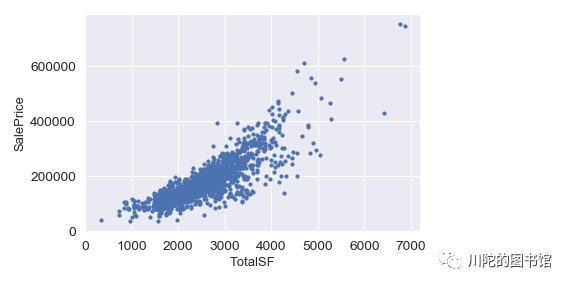
#构造新特征#加地下室面积、1楼面积、2楼面积加起来可以得到房屋总面积特征
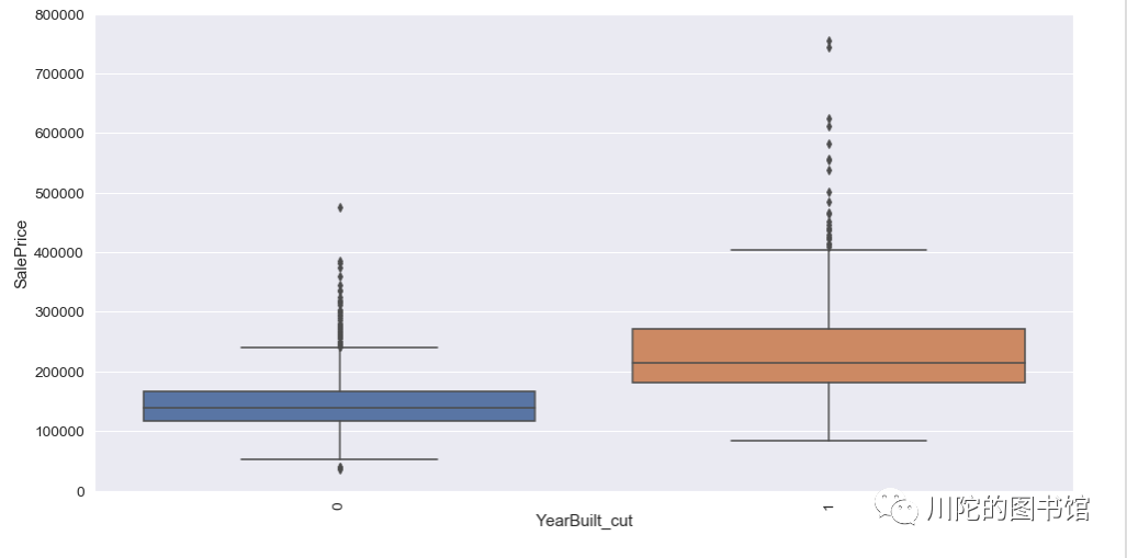
all_data['TotalSF'] = all_data['TotalBsmtSF'] + all_data['1stFlrSF'] + all_data['2ndFlrSF']#之前可视化时候注意到，建造时间比较近的房子房价比较高，#所以新创造一个01特征，如果房屋建造时间在1990年后，则为1，否则是0
all_data['YearBuilt_cut'] = all_data['YearBuilt'].apply(lambda x:1 if x>1990 else 0)

tep = all_data[:ntrain].copy()
tep['SalePrice']=y_train#查看新构造的房屋总面积特征，发现与房价有比较强的线性关系，
fig, ax = plt.subplots()
ax.scatter(tep['TotalSF'], tep['SalePrice'])
plt.ylabel('SalePrice', fontsize=13)
plt.xlabel('TotalSF', fontsize=13)
plt.show()

#建筑年限，可以看到1990年前建造的房子和1990后建造的房子房价在分布上有较大的差异
var = 'YearBuilt_cut'
data = pd.concat([tep['SalePrice'], tep[var]], axis=1)
f, ax = plt.subplots(figsize=(16, 8))
fig = sns.boxplot(x=var, y="SalePrice", data=data)
fig.axis(ymin=0, ymax=800000);
plt.xticks(rotation=90);

对离散变量进行编码处理

from sklearn.preprocessing import LabelEncoder#对有序的离散变量做标签编码#FireplaceQu 壁炉质量#BsmtQual 地下室的高度#BsmtCond 地下室的总体状况#GarageQual 车库质量#GarageCond 车库状况#ExterQual 外部材质的质量#ExterCond 外部材料的现状#HeatingQC 采暖质量和条件#KitchenQual 厨房质量#BsmtFinType1 地下室竣工面积等级#BsmtFinType2 地下室完工区域的等级(如果有多种类型#Functional 家庭功能#BsmtExposure 花园走道的围墙#GarageFinish 车库内部装修#LandSlope 物业坡度#LotShape 房屋的形态#PavedDrive 车道铺面#Street 通往房屋的道路类型#CentralAir 中央空调#MSSubClass 房屋类型(分数标签)#OverallCond 评估房子的整体状况(分数标签)#YrSold 销售年份#MoSold 销售月份
cols = ('FireplaceQu', 'BsmtQual', 'BsmtCond', 'GarageQual', 'GarageCond','ExterQual', 'ExterCond','HeatingQC', 'KitchenQual', 'BsmtFinType1','BsmtFinType2', 'Functional', 'BsmtExposure', 'GarageFinish', 'LandSlope','LotShape', 'PavedDrive', 'Street', 'CentralAir', 'MSSubClass', 'OverallCond','YrSold', 'MoSold')# process columns, apply LabelEncoder to categorical featuresfor c in cols:
    lbl = LabelEncoder()
    lbl.fit(list(all_data[c].values))
    all_data[c] = lbl.transform(list(all_data[c].values))

#数据集中还有部分非有序性离散变量，我们将他们转换成哑变量的形式(和onehot一个意思)
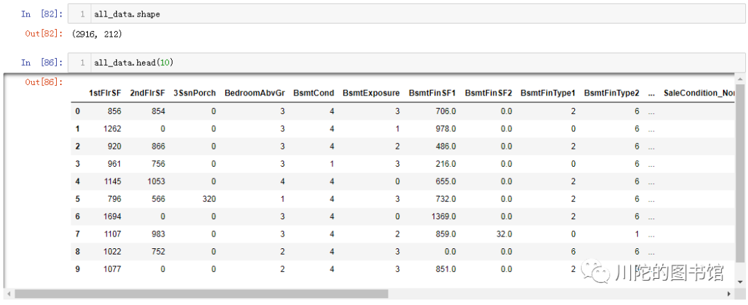
all_data = pd.get_dummies(all_data)

all_data.shape
all_data.head(10)

特征筛选，为避免多重共线性问题，将皮尔森相关性系数大于0.9的特征删除。

threshold = 0.9#相关性矩阵
corr_matrix = all_data.corr().abs()#只选择矩阵的上半部分
upper = corr_matrix.where(np.triu(np.ones(corr_matrix.shape), k=1).astype(np.bool))
upper.head()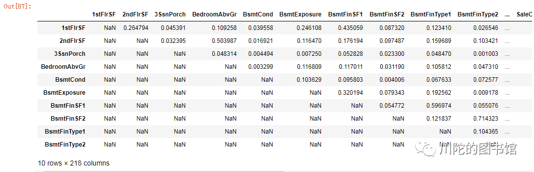

#有6列特征需要删掉
to_drop = [column for column in upper.columns if any(upper[column] > threshold)]
print('There are %d columns to remove.' % (len(to_drop)))
print(to_drop)

all_data = all_data.drop(columns = to_drop)

There are 6 columns to remove.
['Exterior2nd_CmentBd', 'Exterior2nd_MetalSd', 'Exterior2nd_VinylSd', 'GarageType_None', 'RoofStyle_Hip', 'SaleType_New']

#之前是把train和test数据集放在一起进行数据处理，#现在再分开训练集和测试集
train = all_data[:ntrain]
test = all_data[ntrain:]#y_train 采用log对数变换对房价进行处理
y_train= np.log1p(y_train)

四 建模预测

• 岭回归的线性模型

#导入依赖的模块from sklearn.linear_model import Ridgefrom sklearn.model_selection import cross_val_score

使用Sklearn的cross-valu-score函数 (交叉验证) 去作为模型准确性的评估

def rmse_cv(model):    rmse= np.sqrt(-cross_val_score(model, train, y_train, scoring="neg_mean_squared_error", cv = 5)) #cv=5 折叠数    return(rmse)

#导入ridge模型
model_ridge = Ridge()
alphas = [0.05, 0.1, 0.3, 1, 3, 5, 10, 15, 30, 50, 75]# alphas 正则强度
cv_ridge = [rmse_cv(Ridge(alpha = alpha)).mean() for alpha in alphas]

cv_ridge = pd.Series(cv_ridge, index = alphas)
cv_ridge.plot(title = "Validation - Just Do It")
plt.xlabel("alpha")
plt.ylabel("rmse")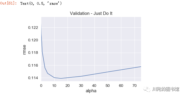

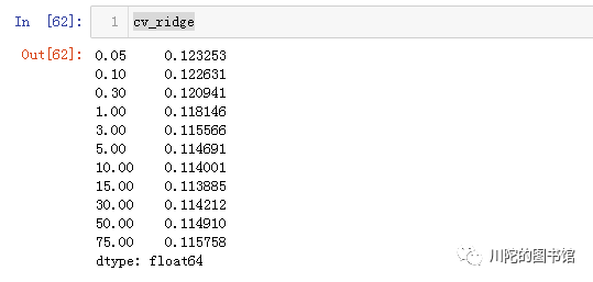
#alpha参数用最优的15,然后用训练集对模型进行训练
clf = Ridge(alpha=15)
clf.fit(train,y_train)

Ridge(alpha=15, copy_X=True, fit_intercept=True, max_iter=None, normalize=False,
      random_state=None, solver='auto', tol=0.001)

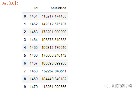
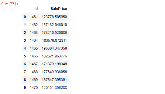
#对测试集预测predict = clf.predict(test)

sub = pd.DataFrame()
sub['Id'] = test_ID#对预测结果做 expm1 对数变换还原
sub['SalePrice']= np.expm1(predict)
sub.to_csv('submission.csv',index=False) #保存结果
sub.head(10)

• 决策树

#导入模块from sklearn.tree import DecisionTreeRegressor

#使用网格搜索法 寻找最佳参数from sklearn.model_selection import GridSearchCV#预设参数选项
max_depth =[18,19,20,21,22]  #最大深度
min_samples_split=[2,4,6,8]  #分裂前节点必须有的最小样本数
min_samples_leaf =[2,4,8,10,12]#分裂前节点加权实例总数的占比
parameters ={'max_depth':max_depth,'min_samples_split':min_samples_split,'min_samples_leaf':min_samples_leaf}#网格搜索
grid_dtcating = GridSearchCV(estimator =DecisionTreeRegressor(),scoring='neg_mean_squared_error',param_grid=parameters,cv=5)#模型拟合
grid_dtcating.fit(train,y_train)#返回最佳组合的参数值
print(grid_dtcating.best_params_)

{'min_samples_leaf': 12, 'max_depth': 18, 'min_samples_split': 8}

#训练
tree_reg = DecisionTreeRegressor(max_depth=21,min_samples_split=6,min_samples_leaf=10)
tree_reg.fit(train,y_train)

DecisionTreeRegressor(ccp_alpha=0.0, criterion='mse', max_depth=21,
           max_features=None, max_leaf_nodes=None,
           min_impurity_decrease=0.0, min_impurity_split=None,
           min_samples_leaf=10, min_samples_split=6,
           min_weight_fraction_leaf=0.0, presort='deprecated',
               random_state=None, splitter='best')

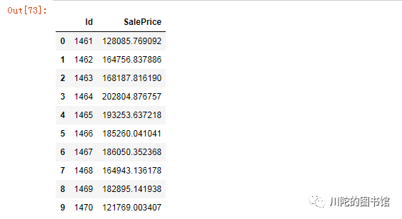
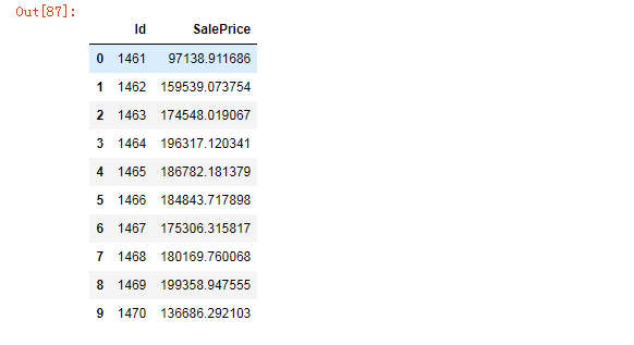
#预测predict_tree = tree_reg.predict(test)

sub_tree = pd.DataFrame()
sub_tree['Id'] = test_ID#对预测结果做 expm1 对数变换还原
sub_tree['SalePrice']= np.expm1(predict_tree)
sub_tree.to_csv('submission_tree.csv',index=False)
sub_tree.head(10)

• 随机森林

#导入模块from sklearn.ensemble import RandomForestRegressor#构造用于回归的随机森林
RF = RandomForestRegressor(n_estimators=200,random_state=451)#随机森林拟合
RF.fit(train,y_train)#进行预测
predict_rf=RF.predict(test)

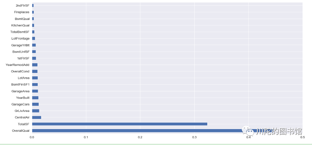
#查看 基于随机森林计算的变量重要性
importance =pd.Series(RF.feature_importances_ ,index=train.columns)
fig, axs = plt.subplots(figsize=(20,10))
importance.sort_values(ascending=False)[:20].plot('barh')
plt.xlim([0,0.5])
plt.show()

sub_tree = pd.DataFrame()
sub_tree['Id'] = test_ID#对预测结果做 expm1 对数变换还原
sub_tree['SalePrice']= np.expm1(predict_rf)
sub_tree.to_csv('submission_rf.csv',index=False)
sub_tree.head(10)

• 梯度提升 Gradient Boosting GBRT 

#导入模块from sklearn.ensemble import GradientBoostingRegressor#使用网格搜索法 寻找最佳参数
learning_rate=[0.05,0.1,0.2] #模型迭代的学习率
n_estimators =[100,200,300] #基础模型的数量
max_depth = [18,19,20,21] #每个模型的最大深度
params ={'learning_rate':learning_rate,'n_estimators':n_estimators,'max_depth':max_depth}
gbdt_grid= GridSearchCV(estimator=GradientBoostingRegressor(),scoring='neg_mean_squared_error',param_grid=params,cv=5)#模型拟合
bdt_grid.fit(train,y_train)#返回最佳组合的参数值
print(gbdt_grid.best_params_)

{'learning_rate': 0.1, 'n_estimators': 300, 'max_depth': 19}

#使用最佳参数训练
predict_gbdt=GradientBoostingRegressor(max_depth=19,n_estimators=300,learning_rate=0.1)
predict_gbdt.fit(train,y_train)

GradientBoostingRegressor(alpha=0.9, ccp_alpha=0.0, criterion='friedman_mse',
             init=None, learning_rate=0.1, loss='ls', max_depth=19,
             max_features=None, max_leaf_nodes=None,
             min_impurity_decrease=0.0, min_impurity_split=None,
             min_samples_leaf=1, min_samples_split=2,
             min_weight_fraction_leaf=0.0, n_estimators=300,
             n_iter_no_change=None, presort='deprecated',
             random_state=None, subsample=1.0, tol=0.0001,
              validation_fraction=0.1, verbose=0, warm_start=False)

#预测
predict_gbdtvalue = predict_gbdt.predict(test)

sub_gbdt = pd.DataFrame()
sub_gbdt['Id'] = test_ID#对预测结果做 expm1 对数变换还原
sub_gbdt['SalePrice']= np.expm1(predict_gbdtvalue)
sub_gbdt.to_csv('submission_gbdt.csv',index=False)
sub_gbdt.head(10)