机器学习学习笔记----LinearRegression,RidgeCV,LassoCV,ElasticNetCV

import numpy as np
from sklearn.linear_model import LinearRegression, RidgeCV, LassoCV, ElasticNetCV
from sklearn.preprocessing import PolynomialFeatures
from sklearn.pipeline import Pipeline
from sklearn.exceptions import ConvergenceWarning
import matplotlib as mpl
import matplotlib.pyplot as plt
import warnings
import seaborn


def xss(y, y_hat):
    y = y.ravel()
    y_hat = y_hat.ravel()
    # Version 1
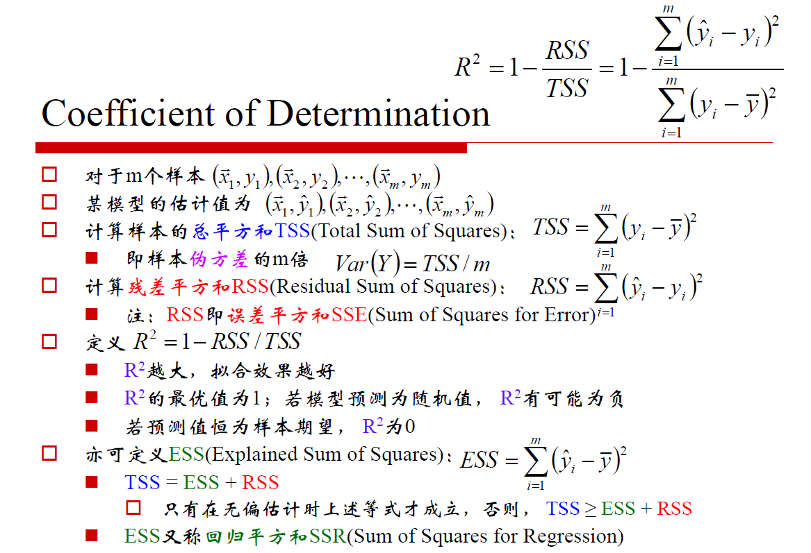
    tss = ((y - np.average(y)) ** 2).sum()
    rss = ((y_hat - y) ** 2).sum()
    ess = ((y_hat - np.average(y)) ** 2).sum()
    r2 = 1 - rss / tss
    # print 'RSS:', rss, '\t ESS:', ess
    # print 'TSS:', tss, 'RSS + ESS = ', rss + ess
    tss_list.append(tss)
    rss_list.append(rss)
    ess_list.append(ess)
    ess_rss_list.append(rss + ess)
    # Version 2
    # tss = np.var(y)
    # rss = np.average((y_hat - y) ** 2)
    # r2 = 1 - rss / tss
    corr_coef = np.corrcoef(y, y_hat)[0, 1]  #协方差
    return r2, corr_coef


if __name__ == "__main__":
    warnings.filterwarnings(action='ignore', category=ConvergenceWarning)
    np.random.seed(0)
    np.set_printoptions(linewidth=300)
    N = 9
    x = np.linspace(0, 6, N) + np.random.randn(N)   #生成带噪声的0-6之间的9个点
    x = np.sort(x)
    y = x**2 - 4*x - 3 + np.random.randn(N)
    #将x,y的维度都变为9x1
    x.shape = -1, 1
    y.shape = -1, 1
    print(y)
# '''
# 线性回归的目的是要得到输出向量Y和输入特征X之间的线性关系,求出线性回归系数θ，也就是Y=Xθ,
# 其中Y的维度为mx1,X的维度为mxn，而θ的维度为nx1,m代表样本个数,n代表样本特征的维度
# 损失函数:损失函数是用来评价模型的预测值f(x)与真实值Y的不一致程度,它是一个非负实值函数 通常用L(Y,f(x))表示,损失函数越小,模型的性能就越好
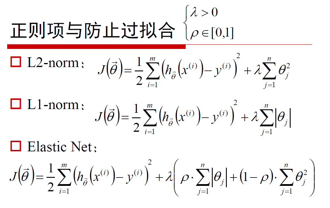
# 正则化项:为了防止损失函数过拟合的问题，一般会在损失函数中加上正则化项,增加模型的泛化能力
# '''

    models = [
        # '''
        # 损失函数:J(θ)=1/2(Xθ−Y)T(Xθ−Y) 优化方法：梯度下降和最小二乘法,scikit中采用最小二乘
        # 使用场景:只要数据线性相关，LinearRegression是我们的首选,如果发现拟合或者预测的不够好，再考虑其他的线性回归库
        # '''
        Pipeline([
        ('poly', PolynomialFeatures()),
        ('linear', LinearRegression(fit_intercept=False))]),
        # '''
        # Ridge回归(岭回归)损失函数的表达形式：J(θ)=1/2(Xθ−Y)T(Xθ−Y)+1/2α||θ||2(线性回归LineaRegression的损失函数+L2（2范式的正则化项）)
        # a为超参数 alphas=np.logspace(-3, 2, 10) 从给定的超参数a中选择一个最优的,logspace用于创建等比数列 本例中 开始点为10的-3次幂,结束点10的2次幂,元素个数为
        # 10,并且从这10个数中选择一个最优的超参数
        # Ridge回归中超参数a和回归系数θ的关系,a越大，正则项惩罚的就越厉害，得到的回归系数θ就越小,最终趋近与0
        # 如果a越小,即正则化项越小，那么回归系数θ就越来越接近于普通的线性回归系数
        # 使用场景:只要数据线性相关，用LinearRegression拟合的不是很好，需要正则化，可以考虑使用RidgeCV回归,
        # 如何输入特征的维度很高,而且是稀疏线性关系的话， RidgeCV就不太合适,考虑使用Lasso回归类家族
        # '''
        Pipeline([
            ('poly', PolynomialFeatures()),
            ('linear', RidgeCV(alphas=np.logspace(-3, 2, 10), fit_intercept=False))]),
        # '''
        # 损失函数:J(θ)=1/2m(Xθ−Y)T(Xθ−Y)+α||θ|| 线性回归LineaRegression的损失函数+L1（1范式的正则化项）)
        # Lasso回归可以使得一些特征的系数变小,甚至还使一些绝对值较小的系数直接变为0，从而增强模型的泛化能力
        # 使用场景:对于高纬的特征数据,尤其是线性关系是稀疏的，就采用Lasso回归,或者是要在一堆特征里面找出主要的特征，那么
        # Lasso回归更是首选了
        # '''
        Pipeline([
            ('poly', PolynomialFeatures()),
            ('linear', LassoCV(alphas=np.logspace(-3, 2, 10), fit_intercept=False))]),
        # '''
        # #损失函数：J(θ)=1/2m(Xθ−Y)T(Xθ−Y)+αρ||θ||+α(1−ρ)/2||θ||2  其中α为正则化超参数，ρ为范数权重超参数
        # #alphas=np.logspace(-3, 2, 10), l1_ratio=[.1, .5, .7, .9, .95, .99, 1] ElasticNetCV会从中选出最优的 a和p
        # #ElasticNetCV类对超参数a和p使用交叉验证，帮助我们选择合适的a和p
        # #使用场景:ElasticNetCV类在我们发现用Lasso回归太过(太多特征被稀疏为0),而Ridge回归也正则化的不够(回归系数衰减太慢)的时候
        # '''
        Pipeline([
            ('poly', PolynomialFeatures()),
            ('linear', ElasticNetCV(alphas=np.logspace(-3, 2, 10), l1_ratio=[.1, .5, .7, .9, .95, .99, 1],
                                    fit_intercept=False))])
    ]
    mpl.rcParams['font.sans-serif'] = ['simHei']
    mpl.rcParams['axes.unicode_minus'] = False
    np.set_printoptions(suppress=True)

    plt.figure(figsize=(18, 12), facecolor='w')
    d_pool = np.arange(1, N, 1)  # 阶array([1, 2, 3, 4, 5, 6, 7, 8])

    m = d_pool.size  #8
    clrs = []  # 颜色
    for c in np.linspace(16711680, 255, m, dtype=int):
        clrs.append('#%06x' % c)
    line_width = np.linspace(5, 2, m)
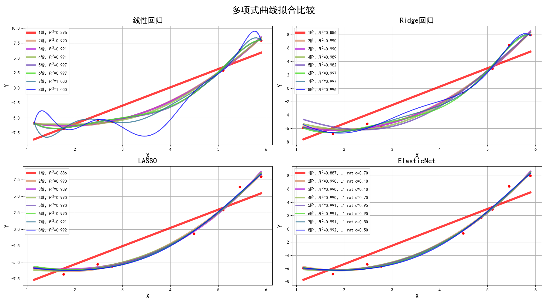
    titles = '线性回归', 'Ridge回归', 'LASSO', 'ElasticNet'
    tss_list = [] #((y - np.average(y)) ** 2).sum()
    rss_list = [] #((y_hat - y) ** 2).sum()
    ess_list = [] #((y_hat - np.average(y)) ** 2).sum()
    ess_rss_list = []
    for t in range(4):
        model = models[t]  #第t个模型，0是LinearRegression，1是RidgeCV，2是LASSO,3是Elastic Net
        plt.subplot(2, 2, t+1)
        #ms点的大小
        plt.plot(x, y, 'ro', ms=5)
        for i, d in enumerate(d_pool): #i[0,1,2,3,4,5,6,7]  d[1,2,3,4,5,6,7,8]
            model.set_params(poly__degree=d)
            model.fit(x, y.ravel())
            lin = model.get_params('linear')['linear']
            output = '%s：%d阶，系数为：' % (titles[t], d)
            if hasattr(lin, 'alpha_'):
                idx = output.find('系数')
                output = output[:idx] + ('alpha=%.6f，' % lin.alpha_) + output[idx:]
            if hasattr(lin, 'l1_ratio_'):   # 根据交叉验证结果，从输入l1_ratio(list)中选择的最优l1_ratio_(float)
                idx = output.find('系数')
                output = output[:idx] + ('l1_ratio=%.6f，' % lin.l1_ratio_) + output[idx:]
            print(output, lin.coef_.ravel())
            x_hat = np.linspace(x.min(), x.max(), num=100)
            print(x_hat)
            x_hat.shape = -1, 1    #100*1
            y_hat = model.predict(x_hat)
            s = model.score(x, y)  #R^2
            r2, corr_coef = xss(y, model.predict(x))
            # print 'R2和相关系数：', r2, corr_coef
            # print 'R2：', s, '\n'
            label = '%d阶，$R^2$=%.3f' % (d, s)
            #print(label)
            if hasattr(lin, 'l1_ratio_'):
                label += '，L1 ratio=%.2f' % lin.l1_ratio_
            plt.plot(x_hat, y_hat, color=clrs[i], lw=line_width[i], alpha=0.75, label=label)
        plt.legend(loc='upper left')
        plt.grid(True)
        plt.title(titles[t], fontsize=18)
        plt.xlabel('X', fontsize=16)
        plt.ylabel('Y', fontsize=16)
    plt.tight_layout(1, rect=(0, 0, 1, 0.95))
    plt.suptitle('多项式曲线拟合比较', fontsize=22)
    plt.show()

    y_max = max(max(tss_list), max(ess_rss_list)) * 1.05
    plt.figure(figsize=(9, 7), facecolor='w')
    t = np.arange(len(tss_list))
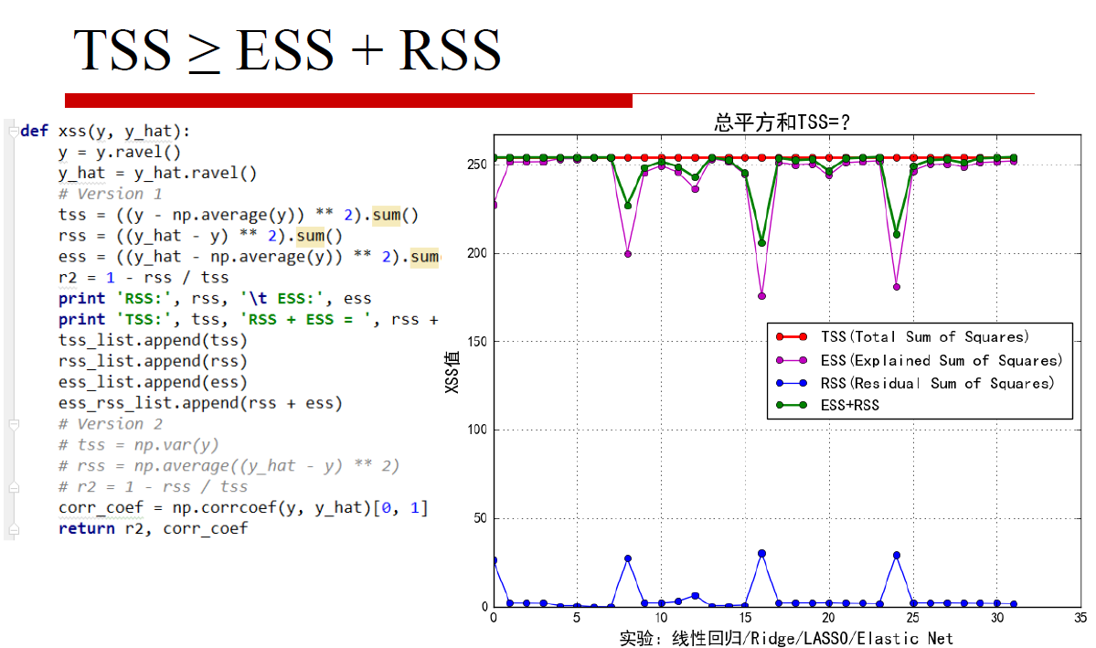
    plt.plot(t, tss_list, 'ro-', lw=2, label='TSS(Total Sum of Squares)')
    plt.plot(t, ess_list, 'mo-', lw=1, label='ESS(Explained Sum of Squares)')
    plt.plot(t, rss_list, 'bo-', lw=1, label='RSS(Residual Sum of Squares)')
    plt.plot(t, ess_rss_list, 'go-', lw=2, label='ESS+RSS')
    plt.ylim((0, y_max))
    plt.legend(loc='center right')
    plt.xlabel('实验：线性回归/Ridge/LASSO/Elastic Net', fontsize=15)
    plt.ylabel('XSS值', fontsize=15)
    plt.title('总平方和TSS=？', fontsize=18)
    plt.grid(True)
    plt.show()