Montecarlo Methods

Montecarlo Methods

1 原理介绍

• key: to estimate the expected values of dependent variables.

1.1 Pseudo-Code 介绍原理

• We do so by drawing a random sample of 𝑛 random numbers, 𝑥1,𝑥2,…,𝑥𝑛, from the specified distribution.
• We map these values onto a sample of the dependent variable 𝑌: 𝑓(𝑥1),𝑓(𝑥2),…,𝑓(𝑥𝑛).
• We can use the sample mean $\bar{y}$=∑𝑛𝑖=1𝑓(𝑥𝑖)/𝑛 to estimate 𝐄[𝑌].
• Provided that 𝑛 is sufficiently large, our estimate will be accurate by the law of large numbers.
• $\bar{y}$ is called the Monte-Carlo estimator.

sample = []
for i in range(n):
	x = draw_random_value(distribution)
	y = f(x)
	sample.append(y)
result = mean(sample)

• We can write this more concisely using a comprehension:

inputs = draw_random_value(distribution, size=n)
result = mean([f(x) for x in inputs])

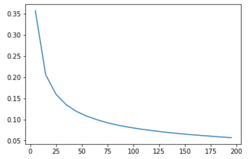
1.2 模拟误差

### 均值误差
mu = 0
def sampling_error(n):
    errors = [np.abs(np.mean(np.random.normal(size=n))- mu) \
              for i in range(100000)]
    return np.mean(errors)    
sampling_error(5)

检验误差和样本数的关系

import matplotlib.pyplot as plt
%matplotlib inline
n = np.arange(5, 200, 10)
plt.plot(n, np.vectorize(sampling_error)(n))

2 模拟应用

2.1 估计$\pi$

import numpy as np

def f(x, y):
    if x*x + y*y < 1:
        return 1.
    else:
        return 0.

n = 1000000
X = np.random.random(size=n)
Y = np.random.random(size=n)
pi_approx = 4 * np.mean([f(x, y) for (x, y) in zip(X,Y)])
print("Pi is approximately %f" % pi_approx)

2.2 结合 map-reduce 估计 $\pi$

samples = 10000
def f(x,y):
    if x**2 + y**2 < 1:
        return 1
    else:
        return 0
    
def sample(p):
    return f(np.random.random(),np.random.random())

reduce(lambda x,y:x+y,(map(sample,[1]*samples)))/samples * 4

2.2 欧式看涨期权-European call option

• 看涨期权：以固定价格（strike price 𝐾）在到期日（maturity date 𝑇）购进一种资产（该资产价格为$S_t$）的权利。一般来说，当证券价格 $S_t$ 小于行使价格 𝐾 时，
• $S_0$ :初始价格 Initial price level of the security .
• $K$: 行使价格 strike price
• $T$: 到期日 maturity date(time to maturity)
• $\sigma$: 底层资产波动率 Volatility of the security.
• $r$:risk-free interest rate.
• payoff = m a x { S T − K , 0 } max\{S_T -K,0\} max{ST​−K,0}

$$S_T=S_{0}exp\{(r-\frac{{\sigma }^2}{2})T+\sigma \varphi \sqrt{T}\}$$

### European Call Option
### non-path-dependent- 一步随机，没有累积过程，直接用参数计算S_T

from numpy import sqrt, exp, cumsum, sum, maximum, mean
from numpy.random import standard_normal

# Parameters
S0 = 100.; K = 105.
T = 1.0
r = 0.02; sigma = 0.1
I = 100000

# Simulate I outcomes 
S = S0 * exp((r - 0.5 * sigma ** 2) * T + sigma * sqrt(T) * 
                          standard_normal(I))

# Calculate the Monte Carlo estimator
C0 = exp(-r * T) * mean(maximum(S - K, 0)) 
print("Estimated present value is %f" % C0)

2.3 亚式看涨期权-Asian (Average Value) Call Option

• 看涨期权：以固定价格（strike price 𝐾）在到期日（maturity date 𝑇）购进一种资产（该资产价格为$S_t$）的权利。一般来说，当证券价格 $S_t$ 小于行使价格 𝐾 时，可以理解成不行权，价值为0
• $S_0$:初始价格 Initial price level of the security.
• $K$: 行使价格 strike price
• $T$: 到期日 maturity date(time to maturity)
• $M$: GBM 步数(number of time steps)
• $\Delta$: 时间间隔 (dt),$\Delta =T/M$
• $\sigma$: 底层资产波动率 Volatility of the security.
• $I$ : $I$ 种 GBM 可能的路径（number of independent realisations）： $I=10^5$ .
• $r$: risk-free interest rate.
• payoff = m a x { S T − K , 0 } max\{S_T -K,0\} max{ST​−K,0}

思想：

• To simulate GBM at 𝑀 evenly spaced time intervals 𝑡𝑖 with Δ=𝑇/𝑀 :

### Asian (Average Value) Call Option -- neet to know values at every time point
### path-dependent - 需要积累，要算均值
from numpy import sqrt, exp, cumsum, sum, maximum, mean
from numpy.random import standard_normal
import numpy as np

# Parameters
S0 = 100.; T = 1.0; K = 50; r = 0.02; sigma = 0.1
M = 200; dt = T / M; I = 100000

def inner_value(S):
    # Intrinsic value for a fixed-strike Asian call option
    # This uses a list comprehension (though there is probably a faster, vectorised way possible)
    return np.array([max(V - K,0) for V in mean(S, axis=0)])

# Simulate I paths with M time steps
S = S0 * exp(cumsum((r - 0.5 * sigma ** 2) * dt + sigma * sqrt(dt) * 
                          standard_normal((M, I)), axis=0))

# Calculate the Monte Carlo estimator
C0 = exp(-r * T) * mean(inner_value(S))
print("Estimated present value is %f" % C0)