A brief overview of Imitation Learning

Reinforcement learning (RL) is one of the most interesting areas of machine learning, where an agent interacts with an environment by following a policy. In each state of the environment, it takes action based on the policy, and as a result, receives a reward and transitions to a new state. The goal of RL is to learn an optimal policy which maximizes the long-term cumulative rewards.

To achieve this, there are several RL algorithms and methods, which use the received rewards as the main approach to approximate the best policy. Generally, these methods perform really well. In some cases, though the teaching process is challenging. This can be especially true in an environment where the rewards are sparse (e.g. a game where we only receive a reward when the game is won or lost). To help with this issue, we can manually design rewards functions, which provide the agent with more frequent rewards. Also, in certain scenarios, there isn’t any direct reward function (e.g. teaching a self-driving vehicle), thus, the manual approach is necessary. However, manually designing a reward function that satisfies the desired behavior can be extremely complicated.

A feasible solution to this problem is imitation learning (IL). In IL instead of trying to learn from the sparse rewards or manually specifying a reward function, an expert (typically a human) provides us with a set of demonstrations. The agent then tries to learn the optimal policy by following, imitating the expert’s decisions.

Basics of Imitation Learning

Generally, imitation learning is useful when it is easier for an expert to demonstrate the desired behavior rather than to specify a reward function which would generate the same behavior or to directly learn the policy. The main component of IL is the environment, which is essentially a Markov Decision Process (MDP). This means that the environment has an S set of states, an A set of actions, a P(s’|s,a) transition model (which is the probability that an action a in the state s leads to state s’ ) and an unknown R(s,a) reward function. The agent performs different actions in this environment based on its π policy. We also have the expert’s demonstrations (which are also known as trajectories) τ = (s0, a0, s1, a1, …) , where the actions are based on the expert’s (“optimal”) π* policy. In some cases, we even “have access” to the expert at training time, which means that we can query the expert for more demonstrations or for evaluation. Finally, the loss function and the learning algorithm are two main components, in which the various imitation learning methods differ from each other.

Behavioral Cloning

The simplest form of imitation learning is behavior cloning (BC), which focuses on learning the expert’s policy using supervised learning. An important example of behavior cloning is ALVINN, a vehicle equipped with sensors, which learned to map the sensor inputs into steering angles and drive autonomously. This project was carried out in 1989 by Dean Pomerleau, and it was also the first application of imitation learning in general.

The way behavioral cloning works is quite simple. Given the expert’s demonstrations, we divide these into state-action pairs, we treat these pairs as i.i.d. examples and finally, we apply supervised learning. The loss function can depend on the application. Therefore, the algorithm is the following:

In some applications, behavioral cloning can work excellently. For the majority of the cases, though, behavioral cloning can be quite problematic. The main reason for this is the i.i.d. assumption: while supervised learning assumes that the state-action pairs are distributed i.i.d., in MDP an action in a given state induces the next state, which breaks the previous assumption. This also means, that errors made in different states add up, therefore a mistake made by the agent can easily put it into a state that the expert has never visited and the agent has never trained on. In such states, the behavior is undefined and this can lead to catastrophic failures.

Behavioral cloning can fail if the agent makes a mistake (source)

Still, behavioral cloning can work quite well in certain applications. Its main advantages are its simplicity and efficiency. Suitable applications can be those, where we don’t need long-term planning, the expert’s trajectories can cover the state space, and where committing an error doesn’t lead to fatal consequences. However, we should avoid using BC when any of these characteristics are true.

Direct Policy Learning (via Interactive Demonstrator)

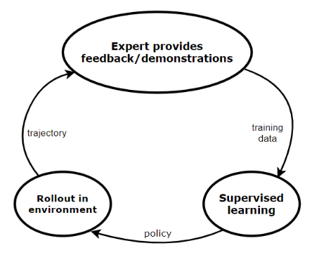
Direct policy learning (DPL) is basically an improved version of behavioral cloning. This iterative method assumes, that we have access to an interactive demonstrator at training time, who we can query. Just like in BC, we collect some demonstrations from the expert, and we apply supervised learning to learn a policy. We roll out this policy in our environment, and we query the expert to evaluate the roll-out trajectory. In this way, we get more training data, which we feedback to supervised learning. This loop continues until we converge.

The general direct policy learning algorithm

The way the general DPL algorithm works is the following. First, we start with an initial predictor policy based on the initial expert demonstrations. Then, we execute a loop until we converge. In each iteration, we collect trajectories by rolling out the current policy (which we obtained in the previous iteration) and using these we estimate the state distribution. Then, for every state, we collect feedback from the expert (what would have he done in the same state). Finally, we train a new policy using this feedback.

To make the algorithm work efficiently, it is important to use all the previous training data during the teaching, so that the agent “remembers” all the mistakes it made in the past. There are several algorithms to achieve this, in this article I introduce two of them: Data Aggregation and Policy Aggregation. Data aggregation trains the actual policy on all the previous training data. Meanwhile, policy aggregation trains a policy on the training data received on the last iteration and then combines this policy with all the previous policies using geometric blending. In the next iteration, we use this newly obtained, blended policy during the roll-out. Both methods are convergent, in the end, we receive a policy which is not much worse than the expert. More information about these methods can be found here.

The full algorithm is the following:

Iterative direct policy learning is a very efficient method, which does not suffer from the problems that BC does. The only limitation of this method is the fact, that we need an expert that can evaluate the agent’s actions at all times, which is not possible in some applications.

Inverse Reinforcement Learning

Inverse reinforcement learning (IRL) is a different approach of imitation learning, where the main idea is to learn the reward function of the environment based on the expert’s demonstrations, and then find the optimal policy (the one that maximizes this reward function) using reinforcement learning. In this approach:

• We start with a set of expert’s demonstrations (we assume these are optimal) and then we try to estimate the parameterized reward function, that would cause the expert’s behavior/policy.

We repeat the following process until we find a good enough policy:

• We update the reward function parameters.
• Then we solve the reinforced learning problem (given the reward function, we try to find the optimal policy).
• Finally, we compare the newly learned policy with the expert’s policy.

The general IRL algorithm is the following:

Depending on the actual problem, there can be two main approaches of IRL: the model-given and the model-free approach. The IRL algorithm of these approaches is different, which is demonstrated in the picture below.

The differences between the model-given and the model-free IRL algorithms

In the model-given case, our reward function is linear. In each iteration, we need to solve the full RL problem, so to be able to do this efficiently, we assume, that the environment’s (the MDP’s) state space is small. We also suppose that we know the state transition dynamics of the environment. This is needed so that we can compare our learned policy with the expert’s one effectively.

The model-free approach is a more general case. Here, we assume that the reward function is more complex, which we usually model with a neural network. We also suppose that the state space of the MDP is large or continuous, therefore in each iteration, we only solve a single step of the RL problem. In this case, we don’t know the state transitions dynamics of the environment, but we assume, that we have access to a simulator or the environment. Therefore, comparing our policy to the expert’s one is trickier.

In both cases, however, learning the reward function is ambiguous. The reason for this is that many rewards functions can correspond to the same optimal policy (the expert’s policy). To solve this issue, we can use the maximum entropy principle proposed by Ziebart: we should choose the trajectory distribution with the largest entropy.

For a better understanding of IRL, more information can be found in these publications:

• Apprenticeship learning via inverse reinforcement learning (Abbeel & Ng, ICML 2004)
• A reduction from apprenticeship learning to classification (Syed & Schapire, NIPS 2010)
• Apprenticeship learning using linear programming (Syed, Bowling & Schapire, ICML 2008)
• Generative adversarial imitation learning (Ho & Ermon, NIPS 2016)
• Guided cost learning: deep inverse optimal control via policy optimization (Finn, Levine & Abbeel, ICML 2016)

Summary

Finally, let’s summarize the imitation learning methods discussed in this article.

Behavioral Cloning:

• advantages: very simple, can be quite efficient in certain applications
• disadvantages: no long-term planning, a mismatch can occur in the state distribution between training and testing (in some applications this can lead to critical failure)
• use when: the application is “simple”, so an error committed by the agent does not lead to severe consequences

Direct Policy Learning:

• advantages: efficient when trained, has long-term planning
• disadvantages: interactive expert/demonstrator is required
• use when: application is more complex and an interactive expert is available

Inverse Reinforced Learning:

• advantages: does not need interactive expert, very efficient when trained (in some cases can outperform the demonstrator), has long-term planning
• disadvantages: can be difficult to train
• use when: application is more complex, an interactive expert is not available or it might be easier to learn the reward functions than the expert’s policy

References

• ICML 2018: Imitation Learning Tutorial (Yisong Yue & Hoang M. Le)
• Imitation learning in large spaces (Stanford University: Reinforcement Learning course)
• A reduction of imitation learning and structured prediction to no-regret online learning (Ross, Gordon & Bagnell, AISTATS 2011)
• Maximum entropy inverse reinforcement learning (Ziebart, Mass, Bagnell & Dey, AAAI 2008)
• Apprenticeship learning via inverse reinforcement learning (Abbeel & Ng, ICML 2004)
• A reduction from apprenticeship learning to classification (Syed & Schapire, NIPS 2010)
• Apprenticeship learning using linear programming (Syed, Bowling & Schapire, ICML 2008)
• Generative adversarial imitation learning (Ho & Ermon, NIPS 2016)
• Guided cost learning: deep inverse optimal control via policy optimization (Finn, Levine & Abbeel, ICML 2016)

Thanks to Robert Moni.

The original post can be read here: https://medium.com/@zoltan.lorincz95/a-brief-overview-of-imitation-learning-25b2a1883f4b