【数据可视化】全球 CO2 浓度展示

---

前言

数据可视化，用到了matplot和cartopy
cartopy文档:https://scitools.org.uk/cartopy/docs/latest/gallery/scalar_data/waves.html#sphx-glr-gallery-scalar-data-waves-py

---

安装cartopy

conda install -c conda-forge cartopy

1.数据

1.1 数据读取

import h5py
import pandas as pd
import numpy as np
import matplotlib.pyplot as plt # plt 用于显示图片
import matplotlib.image as mpimg # mpimg 用于读取图片
import numpy as np

f=h5py.File("./GOSATTFTS2020060120200630_03C01SV0291.h5","r+")
f.keys()
# <KeysViewHDF5 ['Attribute', 'Data', 'Global']>
# 读取所有latitude 纬度信息
dset1 = f["Data"]["geolocation"]["latitude"]
latitude = np.array(dset1)
latitude
###
array([[ 88.75,  88.75,  88.75, ...,  88.75,  88.75,  88.75],
       [ 86.25,  86.25,  86.25, ...,  86.25,  86.25,  86.25],
       [ 83.75,  83.75,  83.75, ...,  83.75,  83.75,  83.75],
       ...,
       [-83.75, -83.75, -83.75, ..., -83.75, -83.75, -83.75],
       [-86.25, -86.25, -86.25, ..., -86.25, -86.25, -86.25],
       [-88.75, -88.75, -88.75, ..., -88.75, -88.75, -88.75]],
      dtype=float32)
###
# 读取所有latitude 纬度信息
dset2 = f["Data"]["geolocation"]["longitude"]
longitude = np.array(dset2)
longitude
###
dset2 = f["Data"]["geolocation"]["longitude"]
longitude = np.array(dset2)
longitude
###

###
###
# 读取所有co2 浓度
dset3 = f["Data"]["mixingRatio"]["XCO2"]
co2 = np.array(dset3)

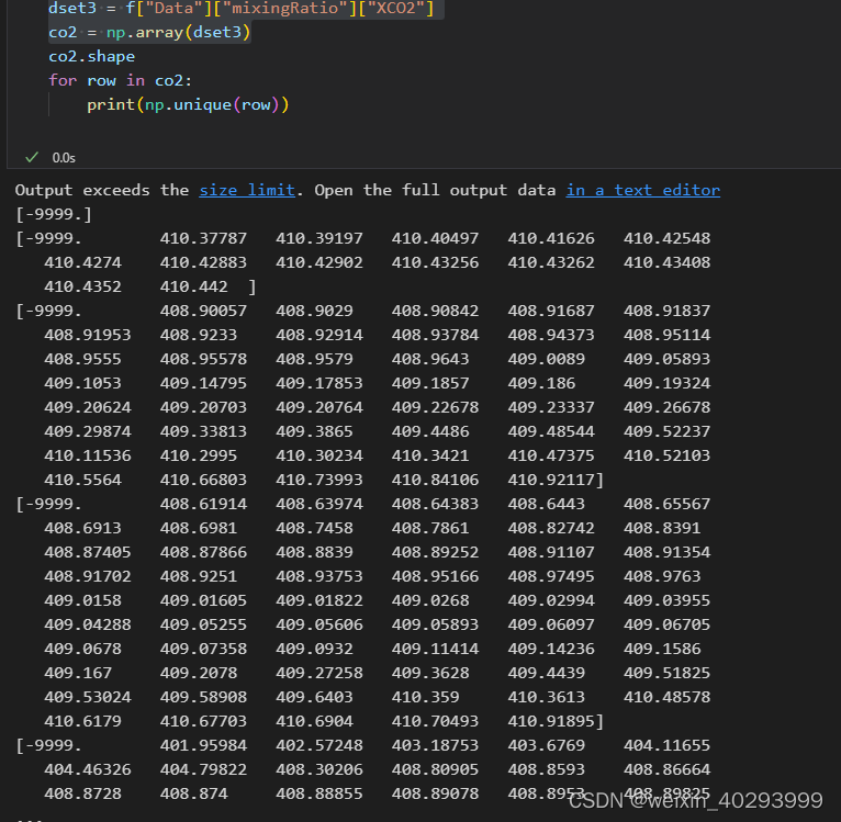
1.2 数据预处理

co2的浓度，-9999时没测到的，

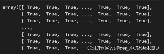
mask = co2 == -9999
mask

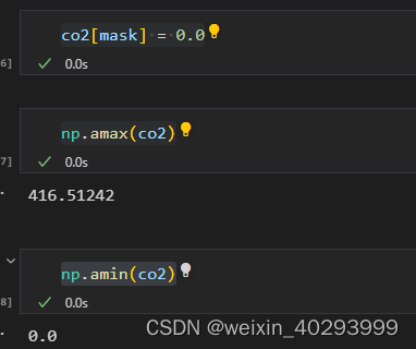
co2[mask] = 0.0

1.3 查看最大，最小值

np.amax(co2)
np.amin(co2)

2.出图

import cartopy.crs as ccrs
from cartopy.mpl.geoaxes import GeoAxes
from cartopy.mpl.ticker import LongitudeFormatter, LatitudeFormatter
import matplotlib.pyplot as plt
from mpl_toolkits.axes_grid1 import AxesGrid
import numpy as np


def sample_data_3d(shape):
    """Return `lons`, `lats`, `times` and fake `data`"""
    ntimes, nlats, nlons = shape
    lats = np.linspace(-np.pi / 2, np.pi / 2, nlats)
    lons = np.linspace(0, 2 * np.pi, nlons)
    lons, lats = np.meshgrid(lons, lats)
    wave = 0.75 * (np.sin(2 * lats) ** 8) * np.cos(4 * lons)
    mean = 0.5 * np.cos(2 * lats) * ((np.sin(2 * lats)) ** 2 + 2)

    lats = np.rad2deg(lats)
    print(lats.shape)
    lons = np.rad2deg(lons)
    data = co2[::-1,:]

    times = np.linspace(-1, 1, ntimes)
    new_shape = data.shape + (ntimes, )
    data = np.rollaxis(data.repeat(ntimes).reshape(new_shape), -1)
    data *= times[:, np.newaxis, np.newaxis]

    return lons, lats, times, data


def main():
    projection = ccrs.PlateCarree()
    axes_class = (GeoAxes,
                  dict(projection=projection))

    lons, lats, times, data = sample_data_3d((6, 72, 144))


    fig = plt.figure(figsize=(10,5))
    axgr = AxesGrid(fig, 111, axes_class=axes_class,
                    nrows_ncols=(1, 1),
                    axes_pad=0.6,
                    cbar_location='right',
                    cbar_mode='single',
                    cbar_pad=0.2,
                    cbar_size='3%',
                    label_mode='')  # note the empty label_mode

    for i, ax in enumerate(axgr):
        if i != 0:
            continue
        ax.coastlines()
        ax.set_xticks(np.linspace(-180, 180, 18), crs=projection)
        ax.set_yticks(np.linspace(-90, 90, 10), crs=projection)
        lon_formatter = LongitudeFormatter(zero_direction_label=True)
        lat_formatter = LatitudeFormatter()
        ax.xaxis.set_major_formatter(lon_formatter)
        ax.yaxis.set_major_formatter(lat_formatter)

        p = ax.contourf(lons, lats, co2[::-1,:],
                        transform=projection,
                        levels=[390, 395, 400, 405, 410, 415],
                        colors=['#80f9ad', '#fff39a', '#ffc512', '#fb7d07', '#E50000']
                )
    

    axgr.cbar_axes[0].colorbar(p)
    ax.axis('off')  # 去掉坐标轴
    plt.savefig("./1.jpg", transparent=True, dpi=300, pad_inches=0, bbox_inches='tight')
    plt.show()
main()

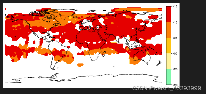
注意点：左下角是数据的起点，所以，我们的co2的数据需要倒置一下。这是一个注意点，否则对不上。