使用keras训练自己的神经网络并在树莓派上运行

最新推荐文章于 2024-06-06 17:13:31 发布

辉映星空

最新推荐文章于 2024-06-06 17:13:31 发布

阅读量1.2w

点赞数 14

文章标签： keras

本文链接：https://blog.csdn.net/weixin_40707450/article/details/79689333

版权

这篇文章主要是使用keras训练一个的识别数字1-46的神经网络并在树莓派上运行的教程。

一、准备数据

数据是自己手动生成的，首先用画图工具生成一个128*128的画布，填充背景为蓝色。

然后用文字工具在画布的中间写数字，我选用的字体是白色，黑体，48，然后保存到文件夹num_data中，并命名为1.png。照这样子画1-64个数字。（呵呵，画了半个小时。。。）

二、扩充训练数据

    到这里为止我们就准备好了原始的数字图片了，但这么少的数字样本肯定不够，我们可以借助keras里面的
图片生成器ImageDataGenerator产生更多的训练样本

首先在工程目录下建一个data文件夹，用来放生成的训练和测试图片

然后编写image_create.py脚本：

#!/usr/bin/env python3
# -*- coding:utf-8 -*-
'''
生成多个样本

author:Administrator
datetime:2018/3/24/024 18:46
software: PyCharm
'''
from keras.preprocessing.image import ImageDataGenerator,array_to_img, img_to_array, load_img
import os


# 生成文件夹
def ensure_dir(dir_path):
    if not os.path.exists(dir_path):
        try:
            os.makedirs(dir_path)
        except OSError:
            pass


# 图片生成器ImageDataGenerator
pic_gen = ImageDataGenerator(
    rotation_range=10,
    width_shift_range=0.1,
    height_shift_range=0.1,
    shear_range=0.2,
    zoom_range=0.2,
    fill_mode='nearest')

# 生成图片
def img_create(img_dir, save_dir, img_prefix, num=100):
    img = load_img(img_dir)
    x = img_to_array(img)
    x = x.reshape((1,) + x.shape)
    img_flow = pic_gen.flow(
        x,
        batch_size=1,
        save_to_dir=save_dir,
        save_prefix=img_prefix,
        save_format="png"
    )
    i = 0
    for batch in img_flow:
        i += 1
        if i > num:
            break


# 生成训练集
for i in range(1, 65, 1):
    img_prefix = str(i)
    img_dir = './num_data/' + img_prefix + '.png'
    save_dir = './data/train/' + img_prefix
    ensure_dir(save_dir)
    img_create(img_dir, save_dir, img_prefix, num=100)
    print("train: ", i)


# 生成测试集
for i in range(1, 65, 1):
    img_prefix = str(i)
    img_dir = './num_data/' + img_prefix + '.png'
    save_dir = './data/validation/' + img_prefix
    ensure_dir(save_dir)
    img_create(img_dir, save_dir, img_prefix, num=50)
    print("validation: ", i)

这个代码主要是构建一个图片生成器，然后生成经过变形的1-64数字图片：

在data文件夹下我们可以看到有两个子文件夹，分别是train和validatin

里面分别是刚刚生成的数据

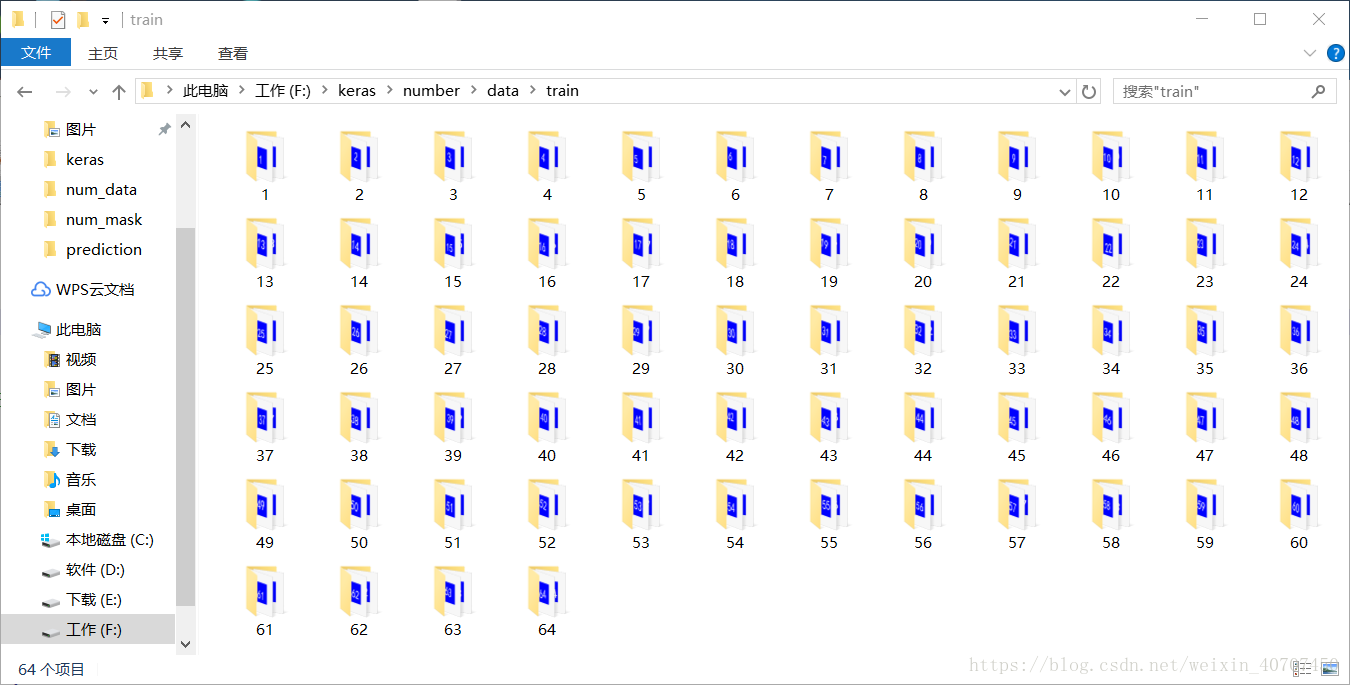
里面就是刚刚生成的数据

三、搭建神经网络训练样本

这次训练采用的是类似VGG的卷积神经网络搭建的模型，通过数据流的方式生成训练样本，这样就可以用cpu来生成数据，用GPU来训练，具体可以参考：flow_from_directory(directory): 以文件夹路径为参数,生成经过数据提升/归一化后的数据,在一个无限循环中无限产生batch数据。图片的大小是128*128彩色图片，

具体的代码：train.py

#!/usr/bin/env python3
# -*- coding:utf-8 -*-
'''
训练数据
author:Administrator
datetime:2018/3/24/024 19:52
software: PyCharm
'''

# 对样本进行预处理
from keras.preprocessing.image import ImageDataGenerator

target = './data/'

# 图片尺寸
img_width, img_height = 128, 128
input_shape = (img_width, img_height, 3)

train_data_dir = target + 'train'
validation_data_dir = target + 'validation'

# 图片生成器ImageDataGenerator
train_pic_gen = ImageDataGenerator(
    rescale=1. / 255,  # 对输入图片进行归一化到0-1区间
    rotation_range=5,
    width_shift_range=0.1,
    height_shift_range=0.1,
    )

# 测试集不做变形处理，只需归一化。
validation_pic_gen = ImageDataGenerator(rescale=1. / 255)

# 按文件夹生成训练集流和标签，
train_flow = train_pic_gen.flow_from_directory(
    train_data_dir,
    target_size=(img_width, img_height),
    batch_size=32,
    # color_mode='grayscale',
    color_mode='rgb',
    classes=[str(i) for i in range(1,65,1)],
    class_mode='categorical')

# 按文件夹生成测试集流和标签，
validation_flow = validation_pic_gen.flow_from_directory(
    validation_data_dir,
    target_size=(img_width, img_height),
    batch_size=32,
    # color_mode='grayscale',
    color_mode='rgb',
    classes=[str(i) for i in range(1,65,1)],
    class_mode='categorical'
)

from keras.models import Sequential
from keras.layers import Conv2D, MaxPooling2D
from keras.layers import Activation, Dropout, Flatten, Dense
from keras.optimizers import SGD
from keras.callbacks import ModelCheckpoint

# 设置训练参数
nb_train_samples = 1000
nb_validation_samples = 100
nb_epoch = 5


# 搭建模型
model = Sequential()

model.add(Conv2D(32, (3, 3), activation='relu', input_shape=input_shape))
model.add(Conv2D(32, (3, 3), activation='relu'))
model.add(MaxPooling2D(pool_size=(2, 2)))
model.add(Dropout(0.25))

model.add(Conv2D(64, (3, 3), activation='relu'))
model.add(Conv2D(64, (3, 3), activation='relu'))
model.add(MaxPooling2D(pool_size=(2, 2)))
model.add(Dropout(0.25))

model.add(Flatten())
model.add(Dense(256, activation='relu'))
model.add(Dropout(0.5))
model.add(Dense(64, activation='softmax'))

sgd = SGD(lr=0.01, decay=1e-6, momentum=0.9, nesterov=True)
model.compile(loss='categorical_crossentropy', optimizer=sgd, metrics=['accuracy'])

model.summary()

# 保存最佳训练参数
checkpointer = ModelCheckpoint(filepath="./tmp/weights.hdf5", verbose=1, save_best_only=True)

model.load_weights('./tmp/weights.hdf5')

# 数据流训练API
model.fit_generator(
    train_flow,
    steps_per_epoch=nb_train_samples,
    epochs=nb_epoch,
    validation_data=validation_flow,
    validation_steps=nb_validation_samples,
    callbacks=[checkpointer]
    )

生成的VGG网络大概是这样子的：

D:\Anaconda2\envs\py36\python.exe F:/keras/number/train.py
Using TensorFlow backend.
Found 12774 images belonging to 64 classes.
Found 6494 images belonging to 64 classes.
_________________________________________________________________
Layer (type) Output Shape Param #
=================================================================
conv2d_1 (Conv2D) (None, 126, 126, 32) 896
_________________________________________________________________
conv2d_2 (Conv2D) (None, 124, 124, 32) 9248
_________________________________________________________________
max_pooling2d_1 (MaxPooling2 (None, 62, 62, 32) 0
_________________________________________________________________
dropout_1 (Dropout) (None, 62, 62, 32) 0
_________________________________________________________________
conv2d_3 (Conv2D) (None, 60, 60, 64) 18496
_________________________________________________________________
conv2d_4 (Conv2D) (None, 58, 58, 64) 36928
_________________________________________________________________
max_pooling2d_2 (MaxPooling2 (None, 29, 29, 64) 0
_________________________________________________________________
dropout_2 (Dropout) (None, 29, 29, 64) 0
_________________________________________________________________
flatten_1 (Flatten) (None, 53824) 0
_________________________________________________________________
dense_1 (Dense) (None, 256) 13779200
_________________________________________________________________
dropout_3 (Dropout) (None, 256) 0
_________________________________________________________________
dense_2 (Dense) (None, 64) 16448
=================================================================
Total params: 13,861,216
Trainable params: 13,861,216
Non-trainable params: 0

_________________________________________________________________

接下来就是漫长的训练咯：

Epoch 1/2

1/1000 [..............................] - ETA: 1:04:16 - loss: 0.2447 - acc: 0.8750
2/1000 [..............................] - ETA: 37:32 - loss: 0.1509 - acc: 0.9219
3/1000 [..............................] - ETA: 34:27 - loss: 0.1233 - acc: 0.9375
4/1000 [..............................] - ETA: 38:28 - loss: 0.1253 - acc: 0.9375
5/1000 [..............................] - ETA: 37:35 - loss: 0.1021 - acc: 0.9500
6/1000 [..............................] - ETA: 39:09 - loss: 0.0983 - acc: 0.9531
7/1000 [..............................] - ETA: 40:36 - loss: 0.0937 - acc: 0.9554
8/1000 [..............................] - ETA: 39:02 - loss: 0.1317 - acc: 0.9570
9/1000 [..............................] - ETA: 36:21 - loss: 0.1297 - acc: 0.9583
10/1000 [..............................] - ETA: 34:53 - loss: 0.1234 - acc: 0.9594
11/1000 [..............................] - ETA: 35:28 - loss: 0.1244 - acc: 0.9574
12/1000 [..............................] - ETA: 34:52 - loss: 0.1243 - acc: 0.9583
13/1000 [..............................] - ETA: 34:08 - loss: 0.1220 - acc: 0.9591
14/1000 [..............................] - ETA: 34:46 - loss: 0.1148 - acc: 0.9621
15/1000 [..............................] - ETA: 33:30 - loss: 0.1127 - acc: 0.9625
16/1000 [..............................] - ETA: 33:11 - loss: 0.1085 - acc: 0.9648
17/1000 [..............................] - ETA: 32:52 - loss: 0.1036 - acc: 0.9651

18/1000 [..............................] - ETA: 32:29 - loss: 0.1091 - acc: 0.9635

。。。。。。

到后面我们可以得到差不多0.98的正确率。在训练过程每一个epoch会保存一次最佳的训练权重到tmp目录下weights.hdf5

四、测试训练效果：

在工程目录下建一个prediction文件夹，放几张待测试的图片：

然后写一个测试代码：predict.py 之间载入刚刚训练好的权重文件，注意修改自己测试的图片的路径

img_path = './prediction/pre0.png'

#!/usr/bin/env python3
# -*- coding:utf-8 -*-
'''
测试模型
author:Administrator
datetime:2018/3/24/024 20:31
software: PyCharm
'''
from keras.models import Sequential
from keras.layers import Conv2D, MaxPooling2D
from keras.layers import Activation, Dropout, Flatten, Dense
from keras.preprocessing import image

from keras.optimizers import SGD

import numpy as np

# 图片尺寸
img_width, img_height = 128, 128
input_shape = (img_width, img_height, 3)
img_path = './prediction/pre0.png'
# img_path = './temp.png'
img = image.load_img(img_path, grayscale=False, target_size=(128, 128))
x = image.img_to_array(img)
x = np.expand_dims(x, axis=0)
x /= 255
print(x.shape)

model = Sequential()

model.add(Conv2D(32, (3, 3), activation='relu', input_shape=input_shape))
model.add(Conv2D(32, (3, 3), activation='relu'))
model.add(MaxPooling2D(pool_size=(2, 2)))
model.add(Dropout(0.25))

model.add(Conv2D(64, (3, 3), activation='relu'))
model.add(Conv2D(64, (3, 3), activation='relu'))
model.add(MaxPooling2D(pool_size=(2, 2)))
model.add(Dropout(0.25))

model.add(Flatten())
model.add(Dense(256, activation='relu'))
model.add(Dropout(0.5))
model.add(Dense(64, activation='softmax'))
model.summary()


sgd = SGD(lr=0.01, decay=1e-6, momentum=0.9, nesterov=True)
model.compile(loss='categorical_crossentropy', optimizer=sgd, metrics=['accuracy'])



# 载入权重
model.load_weights('./tmp/weights.hdf5')

# 进行预测,返回分类结果
classes = model.predict_classes(x)

print(classes+1)

返回的结果是预测的数字。

五、结合opencv来测试

通过opencv从摄像头获取一张图片，然后按下s键抓取图片，丢到上面训练的模型里预测，返回预测的结果：

不多说，直接上代码：test.py:

#!/usr/bin/env python3
# -*- coding:utf-8 -*-
'''
摄像头采集图片验证
author:Administrator
datetime:2018/3/25/025 9:27
software: PyCharm
'''
import cv2

from keras.models import Sequential
from keras.layers import Conv2D, MaxPooling2D
from keras.layers import Activation, Dropout, Flatten, Dense
from keras.preprocessing import image

from keras.optimizers import SGD

import numpy as np

# 图片尺寸
img_width, img_height = 128, 128
input_shape = (img_width, img_height, 3)
# img_path = './prediction/pre0.png'

# 获取图片并进行预处理

def img_pre(img_path = './temp.png'):

    img = image.load_img(img_path, grayscale=False, target_size=(128, 128))
    x = image.img_to_array(img)
    x = np.expand_dims(x, axis=0)
    x /= 255
    # print(x.shape)
    return x

model = Sequential()

model.add(Conv2D(32, (3, 3), activation='relu', input_shape=input_shape))
model.add(Conv2D(32, (3, 3), activation='relu'))
model.add(MaxPooling2D(pool_size=(2, 2)))
model.add(Dropout(0.25))

model.add(Conv2D(64, (3, 3), activation='relu'))
model.add(Conv2D(64, (3, 3), activation='relu'))
model.add(MaxPooling2D(pool_size=(2, 2)))
model.add(Dropout(0.25))

model.add(Flatten())
model.add(Dense(256, activation='relu'))
model.add(Dropout(0.5))
model.add(Dense(64, activation='softmax'))

sgd = SGD(lr=0.01, decay=1e-6, momentum=0.9, nesterov=True)
model.compile(loss='categorical_crossentropy', optimizer=sgd, metrics=['accuracy'])

# 载入权重
model.load_weights('./tmp/weights.hdf5')

cap = cv2.VideoCapture(1)  # 打开usb摄像头
num = ''
while True:
    ret, frame = cap.read()  # 读取一帧图片

    font = cv2.FONT_HERSHEY_SIMPLEX

    k = cv2.waitKey(1)

    if k == ord('s'):  # 如果‘s’键按下，保存图片到电脑

        cv2.imwrite('temp.png', frame)
        x = img_pre()
        # 进行预测,返回分类结果
        classes = model.predict_classes(x)[0]
        num = str(classes + 1)
        print(num)

    elif k == ord('q'):
        break

    cv2.putText(frame, num, (10, 100), font, 4, (0, 0, 255), 2, cv2.LINE_AA) # 在图片上显示预测结果
    cv2.imshow('frame', frame)  # 显示图片

cv2.destroyAllWindows()
cap.release()

效果是这样子的：

没钱买设备，只能用脚架台搭了个测试平台：

六、在树莓派上进行测试：

把刚刚写好的test.py文件和weights.hdf5文件上传到树莓派里面

前提是树莓派要装好opencv3.3、tensorflow1.1.0和keras，用的是python2，教程可以上网搜索，这里就省略了

然后运行在树莓派运行test.py, 按下s键拍照，然后就可以返回预测结果了：

辉映星空

关注

14
点赞
踩
115

收藏

觉得还不错? 一键收藏
5
评论
使用keras训练自己的神经网络并在树莓派上运行

这篇文章主要是使用keras训练一个的识别数字1-46的神经网络并在树莓派上运行的教程。一、准备数据数据是自己手动生成的，首先用画图工具生成一个128*128的画布，填充背景为蓝色。然后用文字工具在画布的中间写数字，我选用的字体是白色，黑体，48，然后保存到文件夹num_data中，并命名为1.png。照这样子画1-64个数字。（呵呵，画了半个小时。。。）二、扩充训练数据 ...
复制链接

扫一扫