从零开始transformers

• home
• blog

TRANSFORMERS FROM SCRATCH

• 18 Aug 2019
• code on github
• video lecture
• 18 Aug 2019 代码在 github 视频讲座

Transformers are a very exciting family of machine learning architectures. Many good tutorials exist (e.g. [1, 2]) but in the last few years, transformers have mostly become simpler, so that it is now much more straightforward to explain how modern architectures work. This post is an attempt to explain directly how modern transformers work, and why, without some of the historical baggage.
转换器是一个非常令人兴奋的机器学习架构家族。存在许多很好的教程（例如[1，2]），但是在过去几年中，变压器大多变得更加简单，因此现在解释现代架构的工作原理更加直接。这篇文章试图直接解释现代变压器是如何工作的，以及为什么，没有一些历史包袱。

I will assume a basic understanding of neural networks and backpropagation. If you’d like to brush up, this lecture will give you the basics of neural networks and this one will explain how these principles are applied in modern deep learning systems.
我将假设对神经网络和反向传播有基本的了解。如果你想复习一下，这个讲座将给你神经网络的基础知识，这个讲座将解释这些原则是如何应用于现代深度学习系统的。

A working knowledge of Pytorch is required to understand the programming examples, but these can also be safely skipped.
理解编程示例需要 Pytorch 的工作知识，但也可以安全地跳过这些示例。

Self-attention 自我关注

The fundamental operation of any transformer architecture is the self-attention operation.
任何变压器架构的基本操作都是自我注意操作。

We'll explain where the name "self-attention" comes from later. For now, don't read too much in to it.
稍后我们将解释“自我注意”这个名字的由来。现在，不要读太多。

Self-attention is a sequence-to-sequence operation: a sequence of vectors goes in, and a sequence of vectors comes out. Let’s call the input vectors 𝐱1,𝐱2,…,𝐱t and the corresponding output vectors 𝐲1,𝐲2,…,𝐲t. The vectors all have dimension k.
自我注意是一种序列到序列的操作：一个向量序列进入，一个向量序列出来。我们将输入向量称为 𝐱1,𝐱2,…,𝐱t ，将相应的输出向量称为 𝐲1,𝐲2,…,𝐲t 。向量都具有 k 维。

To produce output vector 𝐲i, the self attention operation simply takes a weighted average over all the input vectors
为了产生输出向量 𝐲i ，自注意操作只需对所有输入向量取加权平均值

𝐲 i=∑ jw i j𝐱 j.

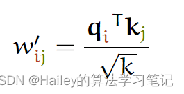
Where j indexes over the whole sequence and the weights sum to one over all j. The weight wij is not a parameter, as in a normal neural net, but it is derived from a function over 𝐱i and 𝐱j. The simplest option for this function is the dot product:
其中 j 表示整个序列的索引，权重之和为一 j 。权重 wij 不是参数，就像在普通神经网络中一样，但它是从 𝐱i 和 𝐱j 上的函数派生的。此函数最简单的选项是点积：

w′ i j=𝐱 iT𝐱 j.

Note that 𝐱i is the input vector at the same position as the current output vector 𝐲i. For the next output vector, we get an entirely new series of dot products, and a different weighted sum.
请注意， 𝐱i 是与当前输出向量 𝐲i 位于同一位置的输入向量。对于下一个输出向量，我们得到一个全新的点积系列，以及一个不同的加权和。

The dot product gives us a value anywhere between negative and positive infinity, so we apply a softmax to map the values to [0,1] and to ensure that they sum to 1 over the whole sequence:
点积为我们提供了一个介于负无穷大和正无穷大之间的值，因此我们应用 softmax 将值映射到 1，并确保它们在整个序列中的总和为 [0,1] ：

w i j=exp w′ i j∑ jexp w′ i j.

And that’s the basic operation of self attention.
这就是自我关注的基本操作。

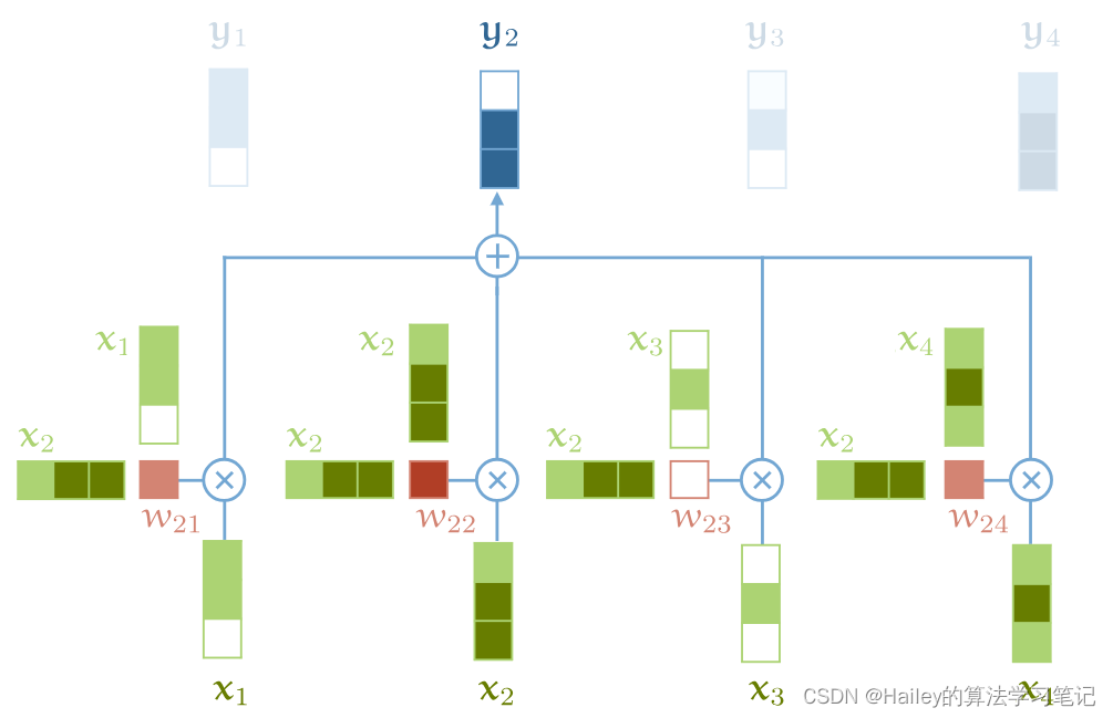
A visual illustration of basic self-attention. Note that the softmax operation over the weights is not illustrated.
基本自我注意的视觉例证。请注意，未说明对权重的 softmax 操作。

A few other ingredients are needed for a complete transformer, which we’ll discuss later, but this is the fundamental operation. More importantly, this is the only operation in the whole architecture that propagates information between vectors. Every other operation in the transformer is applied to each vector in the input sequence without interactions between vectors.
完整的变压器还需要一些其他成分，我们将在后面讨论，但这是基本操作。更重要的是，这是整个架构中唯一在向量之间传播信息的操作。转换器中的所有其他操作都应用于输入序列中的每个向量，而向量之间没有交互。

Understanding why self-attention works
了解为什么自我关注有效

Despite its simplicity, it’s not immediately obvious why self-attention should work so well. To build up some intuition, let’s look first at the standard approach to movie recommendation.
尽管它很简单，但为什么自我关注应该如此有效并不是很明显。为了建立一些直觉，让我们先来看看电影推荐的标准方法。

Let’s say you run a movie rental business and you have some movies, and some users, and you would like to recommend movies to your users that they are likely to enjoy.
假设您经营一家电影租赁业务，您有一些电影和一些用户，并且您想向用户推荐他们可能会喜欢的电影。

One way to go about this, is to create manual features for your movies, such as how much romance there is in the movie, and how much action, and then to design corresponding features for your users: how much they enjoy romantic movies and how much they enjoy action-based movies. If you did this, the dot product between the two feature vectors would give you a score for how well the attributes of the movie match what the user enjoys.
一种方法是为电影创建手动功能，例如电影中有多少浪漫，有多少动作，然后为您的用户设计相应的功能：他们有多喜欢浪漫电影，他们有多喜欢基于动作的电影。如果这样做，两个特征向量之间的点积将为您提供电影属性与用户喜欢的内容匹配程度的分数。

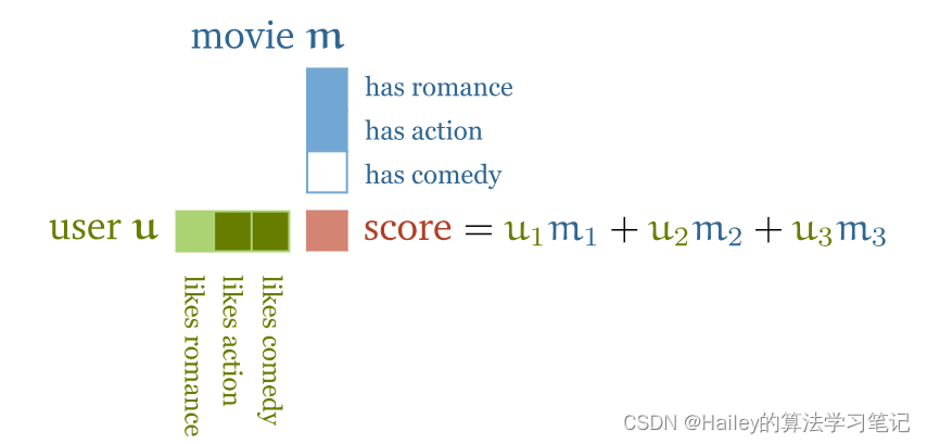
If the signs of a feature match for the user and the movie—the movie is romantic and the user loves romance or the movie is unromantic and the user hates romance—then the resulting dot product gets a positive term for that feature. If the signs don’t match—the movie is romantic and the user hates romance or vice versa—the corresponding term is negative.
如果功能符号与用户和电影匹配（电影是浪漫的，用户喜欢浪漫，或者电影是不浪漫的，用户讨厌浪漫），则生成的点积将获得该功能的正术语。如果符号不匹配（电影是浪漫的，用户讨厌浪漫，反之亦然），则相应的术语是负面的。

Furthermore, the magnitudes of the features indicate how much the feature should contribute to the total score: a movie may be a little romantic, but not in a noticeable way, or a user may simply prefer no romance, but be largely ambivalent.
此外，功能的大小表明该功能对总分的贡献程度：一部电影可能有点浪漫，但并不明显，或者用户可能只是不喜欢浪漫，但在很大程度上是矛盾的。

Of course, gathering such features is not practical. Annotating a database of millions of movies is very costly, and annotating users with their likes and dislikes is pretty much impossible.
当然，收集这些功能是不切实际的。注释包含数百万部电影的数据库非常昂贵，并且几乎不可能用用户的好恶来注释用户。

What happens instead is that we make the movie features and user features parameters of the model. We then ask users for a small number of movies that they like and we optimize the user features and movie features so that their dot product matches the known likes.
相反，我们制作模型的电影功能和用户特征参数。然后，我们要求用户提供少量他们喜欢的电影，并优化用户功能和电影功能，以便他们的点积与已知的喜欢相匹配。

Even though we don’t tell the model what any of the features should mean, in practice, it turns out that after training the features do actually reflect meaningful semantics about the movie content.
尽管我们没有告诉模型任何特征应该意味着什么，但在实践中，事实证明，在训练后，特征确实反映了有关电影内容的有意义的语义。

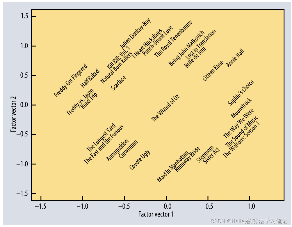
The first two learned features from a basic matrix factorization model. The model had no access to any information about the content of the movies, only which users liked them. Note that movies are arranged from low-brow to high-brow horizontally, and from mainstream to quirky vertically. From [4].
从基本矩阵分解模型中学习的前两个特征。该模型无法访问有关电影内容的任何信息，只能访问哪些用户喜欢它们。请注意，电影是水平从低眉到高眉，从主流到古怪垂直排列的。来自 [4]。

See this lecture for more details on recommender systems. For now, this suffices as an explanation of how the dot product helps us to represent objects and their relations.

This is the basic principle at work in the self-attention. Let’s say we are faced with a sequence of words. To apply self-attention, we simply assign each word t in our vocabulary an embedding vector 𝐯t (the values of which we’ll learn). This is what’s known as an embedding layer in sequence modeling. It turns the word sequence the,cat,walks,on,the,street into the vector sequence
这是自我关注的基本原则。假设我们面对一系列单词。为了应用自我注意，我们只需为词汇表中的每个单词 t 分配一个嵌入向量 𝐯t （我们将学习其值）。这就是序列建模中所谓的嵌入层。它将单词序列 the,cat,walks,on,the,street 转换为向量序列

𝐯 the,𝐯 cat,𝐯 walks,𝐯 on,𝐯 the,𝐯 street.

If we feed this sequence into a self-attention layer, the output is another sequence of vectors
如果我们将此序列馈送到自我注意层中，则输出是另一个向量序列

𝐲 the,𝐲 cat,𝐲 walks,𝐲 on,𝐲 the,𝐲 street

where 𝐲cat is a weighted sum over all the embedding vectors in the first sequence, weighted by their (normalized) dot-product with 𝐯cat.
其中 𝐲cat 是第一个序列中所有嵌入向量的加权和，由它们的（归一化）点积加权 𝐯cat 。

Since we are learning what the values in 𝐯t should be, how "related" two words are is entirely determined by the task. In most cases, the definite article the is not very relevant to the interpretation of the other words in the sentence; therefore, we will likely end up with an embedding 𝐯the that has a low or negative dot product with all other words. On the other hand, to interpret what walks means in this sentence, it's very helpful to work out who is doing the walking. This is likely expressed by a noun, so for nouns like cat and verbs like walks, we will likely learn embeddings 𝐯cat and 𝐯walks that have a high, positive dot product together.
由于我们正在学习 𝐯t 中的值应该是什么，因此两个单词的“相关”程度完全由任务决定。在大多数情况下，定冠词 the 与句子中其他单词的解释不是很相关;因此，我们最终可能会得到一个嵌入 𝐯the ，该嵌入与所有其他单词具有低点积或负点积。另一方面，要解释这句话中走路的意思，弄清楚谁在走路是非常有帮助的。这很可能由名词表达，因此对于像 cat 这样的名词和像 walks 这样的动词，我们可能会学习嵌入 𝐯cat 和 𝐯walks ，它们一起具有高正点积。

This is the basic intuition behind self-attention. The dot product expresses how related two vectors in the input sequence are, with “related” defined by the learning task, and the output vectors are weighted sums over the whole input sequence, with the weights determined by these dot products.

Before we move on, it’s worthwhile to note the following properties, which are unusual for a sequence-to-sequence operation:

• There are no parameters (yet). What the basic self-attention actually does is entirely determined by whatever mechanism creates the input sequence. Upstream mechanisms, like an embedding layer, drive the self-attention by learning representations with particular dot products (although we’ll add a few parameters later).
  （尚）没有参数。基本的自我注意实际上做了什么，完全取决于创建输入序列的任何机制。上游机制，如嵌入层，通过学习特定点积的表示来驱动自我注意力（尽管我们稍后会添加一些参数）。
• Self attention sees its input as a set, not a sequence. If we permute the input sequence, the output sequence will be exactly the same, except permuted also (i.e. self-attention is permutation equivariant). We will mitigate this somewhat when we build the full transformer, but the self-attention by itself actually ignores the sequential nature of the input.
  自我注意将其输入视为一个集合，而不是一个序列。如果我们排列输入序列，输出序列将完全相同，除了排列（即自我注意是排列等变的）。当我们构建完整的转换器时，我们会在一定程度上缓解这一点，但自我关注本身实际上忽略了输入的顺序性质。

In Pytorch: basic self-attention
在 Pytorch 中：基本的自我关注

What I cannot create, I do not understand, as Feynman said. So we’ll build a simple transformer as we go along. We’ll start by implementing this basic self-attention operation in Pytorch.
正如费曼所说，我无法创造的东西，我不理解。因此，我们将构建一个简单的转换器。我们将从在 Pytorch 中实现这个基本的自我注意操作开始。

The first thing we should do is work out how to express the self attention in matrix multiplications. A naive implementation that loops over all vectors to compute the weights and outputs would be much too slow.

我们应该做的第一件事是弄清楚如何在矩阵乘法中表达自我注意。循环遍历所有向量以计算权重和输出的朴素实现太慢了。

We’ll represent the input, a sequence of t vectors of dimension k as a t by k matrix 𝐗. Including a minibatch dimension b, gives us an input tensor of size (b,t,k).

我们将输入表示为输入，一个维度为 k 的 t 向量序列，作为 t x k 矩阵 𝐗 。包括一个小批量维度 10 11，为我们提供了一个大小为 12 13 的输入张量。

The set of all raw dot products w′ij forms a matrix, which we can compute simply by multiplying 𝐗 by its transpose:

所有原始点积 w′ij 的集合形成一个矩阵，我们可以简单地通过将 𝐗 乘以其转置来计算它：

import torch
import torch.nn.functional as F

# assume we have some tensor x with size (b, t, k)
x = ...

raw_weights = torch.bmm(x, x.transpose(1, 2))
# - torch.bmm is a batched matrix multiplication. It
#   applies matrix multiplication over batches of
#   matrices.

Then, to turn the raw weights w′ij into positive values that sum to one, we apply a row-wise softmax:

然后，要将原始权重 w′ij 转换为总和为 1 的正值，我们应用逐行 softmax：

weights = F.softmax(raw_weights, dim=2)

Finally, to compute the output sequence, we just multiply the weight matrix by 𝐗. This results in a batch of output matrices 𝐘 of size (b, t, k) whose rows are weighted sums over the rows of 𝐗.

最后，为了计算输出序列，我们只需将权重矩阵乘以 𝐗 。这将生成一批大小为 (b, t, k) 的输出矩阵 𝐘 ，其行在 𝐗 的行上加权和。

y = torch.bmm(weights, x)

That’s all. Two matrix multiplications and one softmax gives us a basic self-attention.

就这样。两个矩阵乘法和一个softmax给了我们基本的自我关注。

Additional tricks其他技巧

The actual self-attention used in modern transformers relies on three additional tricks.

现代变压器中使用的实际自我注意依赖于三个额外的技巧。

1) Queries, keys and values

1） 查询、键和值

Every input vector 𝐱i is used in three different ways in the self attention operation:

每个输入向量 𝐱i 在自我注意操作中以三种不同的方式使用：

• It is compared to every other vector to establish the weights for its own output 𝐲i
  将其与其他向量进行比较，以建立其自身输出的权重 𝐲i
• It is compared to every other vector to establish the weights for the output of the j-th vector 𝐲j
  将其与其他向量进行比较，以确定 第 1 个向量 𝐲j 的输出权重
• It is used as part of the weighted sum to compute each output vector once the weights have been established.
  它被用作加权和的一部分，以便在建立权重后计算每个输出向量。

These roles are often called the query, the key and the value (we'll explain where these names come from later). In the basic self-attention we've seen so far, each input vector must play all three roles. We make its life a little easier by deriving new vectors for each role, by applying a linear transformation to the original input vector. In other words, we add three k×k weight matrices 𝐖q, 𝐖k,𝐖v and compute three linear transformations of each xi, for the three different parts of the self attention:

这些角色通常称为查询、键和值（稍后我们将解释这些名称的来源）。在我们目前看到的基本自我注意中，每个输入向量必须扮演所有三个角色。我们通过为每个角色推导新的向量，通过将线性变换应用于原始输入向量，使其生活更轻松一些。换句话说，我们添加三个 k×k 权重矩阵 𝐖q 、 𝐖k 、 𝐖v ，并计算每个 xi 的三个线性变换，用于自我注意的三个不同部分：

𝐪 i=𝐖q𝐱 i𝐤 i=𝐖k𝐱 i𝐯 i=𝐖v𝐱 i

w′ i jw i j𝐲 i=𝐪 iT𝐤 j=softmax(w′ i j)=∑ jw i j𝐯 j.

This gives the self-attention layer some controllable parameters, and allows it to modify the incoming vectors to suit the three roles they must play.

这为自我注意层提供了一些可控的参数，并允许它修改传入的向量以适应它们必须扮演的三个角色。

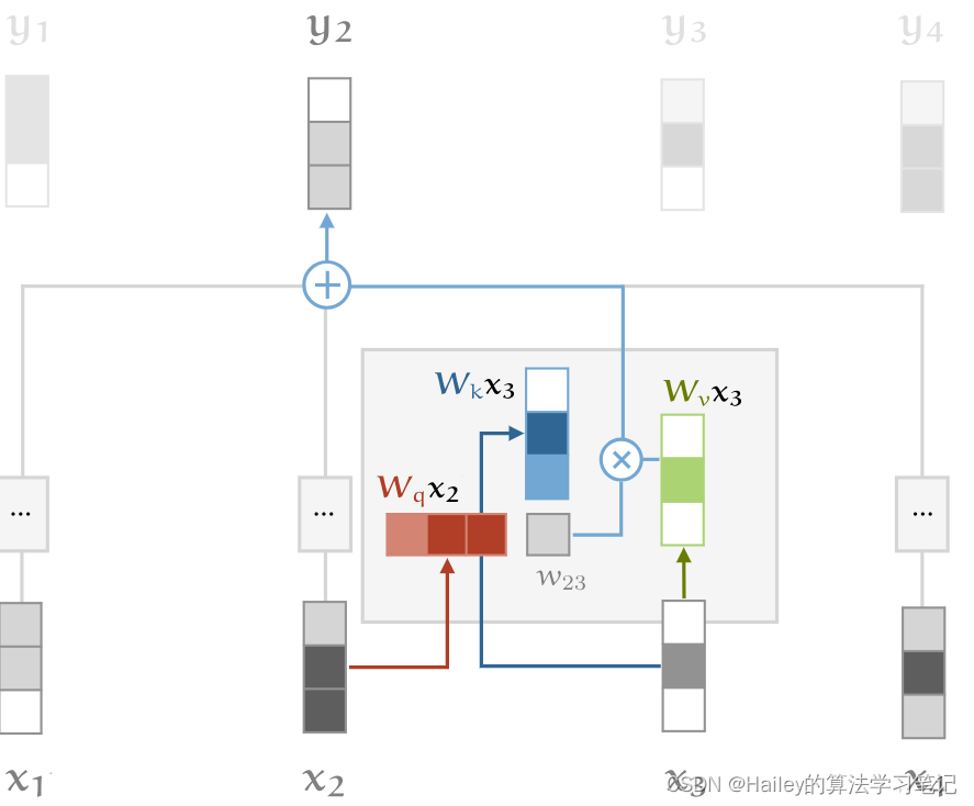
Illustration of the self-attention with key, query and value transformations.

通过键、查询和值转换来说明自我注意。

2) Scaling the dot product缩放点积

The softmax function can be sensitive to very large input values. These kill the gradient, and slow down learning, or cause it to stop altogether. Since the average value of the dot product grows with the embedding dimension k, it helps to scale the dot product back a little to stop the inputs to the softmax function from growing too large:

softmax 函数可能对非常大的输入值敏感。这些会杀死梯度，减慢学习速度，或导致它完全停止。由于点积的平均值随嵌入维度 k 而增长，因此将点积缩小一点有助于阻止 softmax 函数的输入增长过大：

Why k−−√? Imagine a vector in ℝk with values all c. Its Euclidean length is k−−√c. Therefore, we are dividing out the amount by which the increase in dimension increases the length of the average vectors.

为什么是 根号下k？想象一个 ℝk 中的向量，其值全部为 c 。它的欧几里得长度是根号下k 。因此，我们正在除以维数增加平均向量长度的量。

3) Multi-head attention多头注意力

Finally, we must account for the fact that a word can mean different things to different neighbours. Consider the following example.

最后，我们必须考虑到这样一个事实，即一个词对不同的邻居来说可能意味着不同的东西。请考虑以下示例。

mary, gave, roses, to, susan

We see that the word gave has different relations to different parts of the sentence. mary expresses who’s doing the giving, roses expresses what’s being given, and susan expresses who the recipient is.

我们看到，“给予”这个词与句子的不同部分有不同的关系。瑪麗表達誰在做給予，玫瑰表達給予的，蘇珊表達接受者是誰。

In a single self-attention operation, all this information just gets summed together. The inputs 𝐱mary and 𝐱susan can influence the output 𝐲gave by different amounts, depending on their dot-product with 𝐱gave, but they can’t influence it in different ways. If, for instance, we want the information about who gave the roses and who received them to end up in different parts of 𝐲gave, we need a little more flexibility.

在一次自我注意操作中，所有这些信息只是汇总在一起。输入 𝐱mary 和 𝐱susan 可以通过不同的量影响输出 𝐲gave ，具体取决于它们与 𝐱gave 的点积，但它们不能以不同的方式影响它。例如，如果我们希望有关谁送玫瑰和谁收到玫瑰的信息最终出现在 9 的不同部分，我们需要更多的灵活性。

This leaves aside how we figure out who gave the roses. We can do that based on prior knowledge about Mary and Susan, encoded in the embeddings. We can also look at the order of the words, but we'll look at how to achieve that later.
这撇开了我们如何弄清楚谁给了玫瑰。我们可以根据嵌入中编码的有关玛丽和苏珊的先验知识来做到这一点。我们也可以查看单词的顺序，但我们稍后会看看如何实现这一点。

We can give the self attention greater power of discrimination, by combining several self-attention mechanisms (which we'll index with r), each with different matrices 𝐖rq, 𝐖rk,𝐖rv. These are called attention heads.
我们可以通过组合几种自我注意机制（我们将用 r 索引）来赋予自我注意更大的辨别能力，每种机制都有不同的矩阵 𝐖rq ， 𝐖rk ， 𝐖rv 。这些被称为注意力头。

For input 𝐱i each attention head produces a different output vector 𝐲ri. We concatenate these, and pass them through a linear transformation to reduce the dimension back to k.
对于输入 𝐱i ，每个注意头产生不同的输出向量2 𝐲ri 。我们将它们连接起来，并通过线性变换将它们传递回 k 。

Efficient multi-head self-attention. The simplest way to understand multi-head self-attention is to see it as a small number of copies of the self-attention mechanism applied in parallel, each with their own key, value and query transformation. This works well, but for R heads, the self-attention operation is R times as slow.
高效的多头自我关注。理解多头自我注意的最简单方法是将其视为并行应用的自我注意机制的少量副本，每个副本都有自己的键、值和查询转换。这很好用，但对于 R 头，自我注意操作慢了 R 倍。

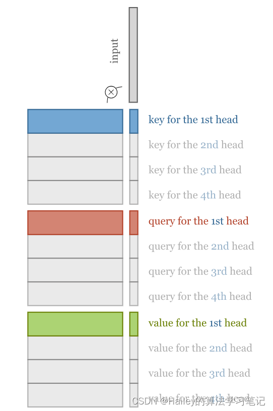
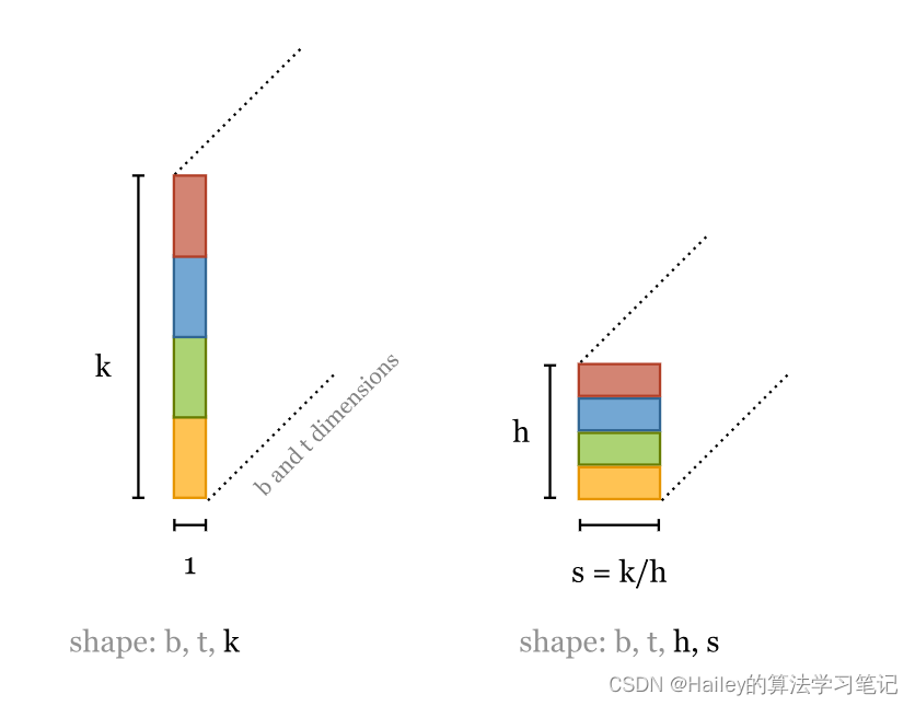
It turns out we can have our cake and eat it too: there is a way to implement multi-head self-attention so that it is roughly as fast as the single-head version, but we still get the benefit of having different self-attention operations in parallel. To accomplish this, each head receives low-dimensional keys queries and values. If the input vector has k=256 dimensions, and we have h=4 attention heads, we multiply the input vectors by a 256×64 matrix to project them down to a sequence of 64 dimansional vectors. For every head, we do this 3 times: for the keys, the queries and the values.
事实证明，我们也可以吃蛋糕：有一种方法可以实现多头自我注意，使其大致与单头版本一样快，但我们仍然可以并行进行不同的自我注意操作。为此，每个头都会接收低维键查询和值。如果输入向量有 k=256 维，我们有 h=4 个注意力头，我们将输入向量乘以 256×64 矩阵，将它们投影到 64 个二元向量的序列中。对于每个头部，我们执行此操作 3 次：键、查询和值。

Here is the whole process illustrated in one image.

这是一张图片中说明的整个过程。

 

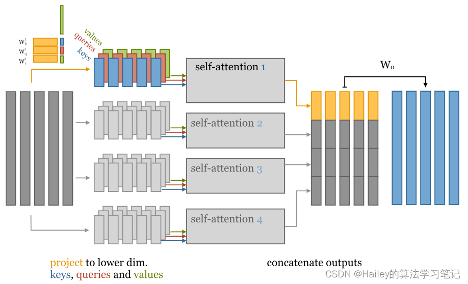
The basic idea of multi-head self-attention with 4 heads. To get our keys, queries and values, we project the input down to vector sequences of smaller dimension.

多头自我注意的基本思想与4个头。为了获取我们的键、查询和值，我们将输入向下投影到较小维度的向量序列。

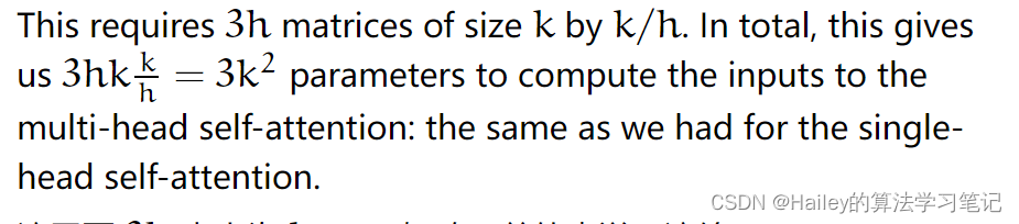
 这需要 3h 大小为 k x 5 的矩阵。总的来说，这给了我们 6 3hkkh=3k2 个参数来计算多头自我注意的输入：与单头自我注意相同。

The only difference is the matrix Wo, used at the end of the multi-head self attention. This adds k^2 parameters compared to the single-head version. In most transformers, the first thing that happens after each self attention is a feed-forward layer, so this may not be strictly necessary. I've never seen a proper ablation to test whether Wo can be removed.

唯一的区别是矩阵 Wo ，用于多头自我注意的末尾。与单头版本相比，这增加了 k^2 个参数。在大多数变压器中，每次自我注意后发生的第一件事就是前馈层，因此这可能不是绝对必要的。我从未见过适当的消融来测试是否可以去除 Wo 。

We can even implement this with just three k×k matrix multiplications as in the single-head self-attention. The only extra operation we need is to slice the resulting sequence of vectors into chunks.

我们甚至可以像单头自我注意一样，只需三个 k×k 矩阵乘法即可实现这一点。我们唯一需要的额外操作是将生成的向量序列切成块

To compute multi-head attention efficiently, we combine the computation of the projections down to a lower dimensional representation and the computations of the keys, queries and values into three k×k matrices.

为了有效地计算多头注意力，我们将投影的计算组合到较低维度的表示中，并将键、查询和值的计算组合成三个 k×k 矩阵。

In Pytorch: complete self-attention在 Pytorch 中：完全的自我关注

Let’s now implement a self-attention module with all the bells and whistles. We’ll package it into a Pytorch module, so we can reuse it later.

现在让我们实现一个包含所有花里胡哨的自我注意模块。我们将它打包到 Pytorch 模块中，以便稍后重用它。

import torch
from torch import nn
import torch.nn.functional as F

class SelfAttention(nn.Module):
    def __init__(self, k, heads=4, mask=False):
      
    super().__init__()
    
    assert k % heads == 0
    
    self.k, self.heads = k, heads

Note the assert: the embedding dimension needs to be divisible by the number of heads.

请注意断言：嵌入维度需要能被头部数量整除。

Next, we set up some linear transformations with emb by emb matrices. The nn.Linear module with the bias disabled gives us such a projection, and provides a reasonable initialization for us.

接下来，我们用 emb x emb 矩阵设置一些线性变换。禁用偏置的 nn.Linear 个模块为我们提供了这样的投影，并为我们提供了合理的初始化。

    
    # These compute the queries, keys and values for all
    # heads
    self.tokeys    = nn.Linear(k, k, bias=False)
    self.toqueries = nn.Linear(k, k, bias=False)
    self.tovalues  = nn.Linear(k, k, bias=False)

	# This will be applied after the multi-head self-attention operation.
    self.unifyheads = nn.Linear(k, k)

We can now implement the computation of the self-attention (the module’s forward function). First, we compute the queries, keys and values for all heads:

现在我们可以实现自我注意的计算（模块的 forward 函数）。首先，我们计算所有头部的查询、键和值：

  def forward(self, x):

    b, t, k = x.size()
    h = self.heads

    queries = self.toqueries(x)
    keys    = self.tokeys(x)   
    values  = self.tovalues(x)

This gives us three vector sequences of the full embedding dimension k. As we saw above we can now cut these into h chunks. we can do this with a simple view operation:
这给了我们三个完全嵌入维度为 k 的向量序列。正如我们在上面看到的，我们现在可以将这些切成 h 块。我们可以通过一个简单的视图操作来做到这一点：

	s = k // h

	keys    = keys.view(b, t, h, s)
	queries = queries.view(b, t, h, s)
	values  = values.view(b, t, h, s)

This simply reshapes the tensors to add a dimension that iterations over the heads. For a single vector in our sequence you can think of it as reshaping a vector of dimension k into a matrix of h by k//h:
这只是重塑张量，以添加一个在头部迭代的维度。对于我们序列中的单个向量，您可以将其视为将维度为 k 的向量重塑为 h x k//h 的矩阵：

 Next, we need to compute the dot products. This is the same operation for every head, so we fold the heads into the batch dimension. This ensures that we can use torch.bmm() as before, and the whole collection of keys, queries and values will just be seen as a slightly larger batch.
接下来，我们需要计算点积。这是每个头部的相同操作，因此我们将头部折叠到批处理维度中。这确保了我们可以像以前一样使用 torch.bmm() ，并且整个键、查询和值的集合将被视为一个稍大的批次。

Since the head and batch dimension are not next to each other, we need to transpose before we reshape. (This is costly, but it seems to be unavoidable.)
由于头部和批次尺寸不相邻，因此我们需要在重塑之前进行转置。（这很昂贵，但似乎是不可避免的。

    # - fold heads into the batch dimension
    keys = keys.transpose(1, 2).contiguous().view(b * h, t, s)
    queries = queries.transpose(1, 2).contiguous().view(b * h, t, s)
    values = values.transpose(1, 2).contiguous().view(b * h, t, s)

You can avoid these calls to contiguous() by using reshape() instead of view() but I prefer to make it explicit when we are copying a tensor, and when we are just viewing it. See this notebook for an explanation of the difference.

你可以通过使用 reshape() 而不是 view() 来避免这些对 contiguous() 的调用，但我更喜欢在我们复制张量时以及当我们只是查看它时明确表示。有关差异的说明，请参阅此笔记本。

As before, the dot products can be computed in a single matrix multiplication, but now between the queries and the keys.
和以前一样，点积可以在单个矩阵乘法中计算，但现在在查询和键之间计算。

   
    # Get dot product of queries and keys, and scale
    dot = torch.bmm(queries, keys.transpose(1, 2))
    # -- dot has size (b*h, t, t) containing raw weights

    # scale the dot product
    dot = dot / (k ** (1/2))
	
    # normalize 
    dot = F.softmax(dot, dim=2)
    # - dot now contains row-wise normalized weights

We apply the self attention weights dot to the values, giving us the output for each attention head
我们将自我注意力权重 dot 应用于值，为我们提供每个注意力头的输出

    
    # apply the self attention to the values
    out = torch.bmm(dot, values).view(b, h, t, s)

To unify the attention heads, we transpose again, so that the head dimension and the embedding dimension are next to each other, and reshape to get concatenated vectors of dimension e. We then pass these through the unifyheads layer for a final projection.
为了统一注意力头，我们再次转置，使头部维度和嵌入维度彼此相邻，并重塑以获得维度为 0 的级联向量。然后，我们将这些通过 unifyheads 层进行最终投影。

    # swap h, t back, unify heads
    out = out.transpose(1, 2).contiguous().view(b, t, s * h)
    
    return self.unifyheads(out)

And there you have it: multi-head, scaled dot-product self attention. You can see the complete implementation here.
这就是：多头，缩放的点积自我关注。您可以在此处查看完整的实现。

The implementation can be made more concise using einsum notation (see an example here).
可以使用 einsum 表示法使实现更加简洁（请参阅此处的示例）。

Building transformers 建筑变压器

A transformer is not just a self-attention layer, it is an architecture. It’s not quite clear what does and doesn’t qualify as a transformer, but here we’ll use the following definition:
变压器不仅仅是一个自我关注层，它是一个架构。目前还不清楚什么符合变压器的条件，什么不符合，但在这里我们将使用以下定义：

Any architecture designed to process a connected set of units—such as the tokens in a sequence or the pixels in an image—where the only interaction between units is through self-attention.
任何旨在处理一组连接的单元（例如序列中的标记或图像中的像素）的体系结构，其中单元之间的唯一交互是通过自我注意。

As with other mechanisms, like convolutions, a more or less standard approach has emerged for how to build self-attention layers up into a larger network. The first step is to wrap the self-attention into a block that we can repeat.
与其他机制一样，如卷积，已经出现了一种或多或少的标准方法，用于如何将自我注意层构建到更大的网络中。第一步是将自我注意力包裹成一个我们可以重复的块。

The transformer block

There are some variations on how to build a basic transformer block, but most of them are structured roughly like this:
关于如何构建一个基本的变压器块有一些变化，但大多数结构大致如下：

 That is, the block applies, in sequence: a self attention layer, layer normalization, a feed forward layer (a single MLP applied independently to each vector), and another layer normalization. Residual connections are added around both, before the normalization. The order of the various components is not set in stone; the important thing is to combine self-attention with a local feedforward, and to add normalization and residual connections.
也就是说，该块按顺序应用：自注意层、层归一化、前馈层（单个 MLP 独立应用于每个向量）和另一层归一化。在规范化之前，在两者周围添加残差连接。各种组件的顺序不是一成不变的;重要的是将自我注意与局部前馈相结合，并添加规范化和残差连接。

Normalization and residual connections are standard tricks used to help deep neural networks train faster and more accurately. The layer normalization is applied over the embedding dimension only.
归一化和残差连接是用于帮助深度神经网络更快、更准确地训练的标准技巧。层规范化仅应用于嵌入维度。

Here’s what the transformer block looks like in pytorch.
这是变压器块在 pytorch 中的样子。

class TransformerBlock(nn.Module):
  def __init__(self, k, heads):
    super().__init__()

    self.attention = SelfAttention(k, heads=heads)

    self.norm1 = nn.LayerNorm(k)
    self.norm2 = nn.LayerNorm(k)

    self.ff = nn.Sequential(
      nn.Linear(k, 4 * k),
      nn.ReLU(),
      nn.Linear(4 * k, k))

  def forward(self, x):
    attended = self.attention(x)
    x = self.norm1(attended + x)

    fedforward = self.ff(x)
    return self.norm2(fedforward + x)

We’ve made the relatively arbitrary choice of making the hidden layer of the feedforward 4 times as big as the input and output. Smaller values may work as well, and save memory, but it should be bigger than the input/output layers.
我们做出了相对任意的选择，使前馈的隐藏层是输入和输出的 4 倍。较小的值也可以工作，并节省内存，但它应该大于输入/输出层。

Classification transformer
分类变压器

The simplest transformer we can build is a sequence classifier. We’ll use the IMDb sentiment classification dataset: the instances are movie reviews, tokenized into sequences of words, and the classification labels are positive and negative (indicating whether the review was positive or negative about the movie).
我们可以构建的最简单的转换器是序列分类器。我们将使用 IMDb 情绪分类数据集：实例是电影评论，标记为单词序列，分类标签为 positive 和 negative （指示评论对电影是正面还是负面）。

The heart of the architecture will simply be a large chain of transformer blocks. All we need to do is work out how to feed it the input sequences, and how to transform the final output sequence into a a single classification.
该架构的核心将只是一个大型变压器块链。我们需要做的就是弄清楚如何向它提供输入序列，以及如何将最终的输出序列转换为单个分类。

The whole experiment can be found here. We won’t deal with the data wrangling in this blog post. Follow the links in the code to see how the data is loaded and prepared.
整个实验可以在这里找到。我们不会在这篇博文中处理数据争吵。按照代码中的链接查看如何加载和准备数据。

Output: producing a classification
输出：生成分类

The most common way to build a sequence classifier out of sequence-to-sequence layers, is to apply global average pooling to the final output sequence, and to map the result to a softmaxed class vector.
从序列到序列层构建序列分类器的最常见方法是将全局平均池化应用于最终输出序列，并将结果映射到softmaxed类向量。

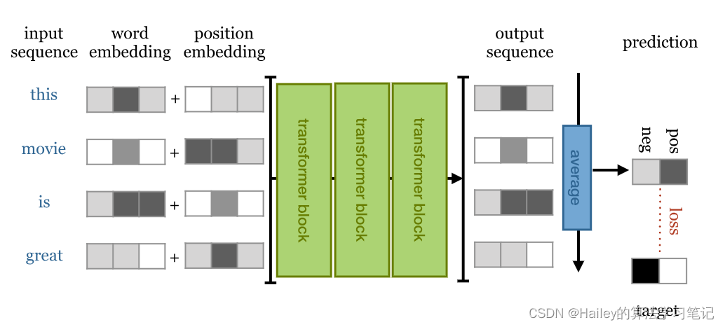
 Overview of a simple sequence classification transformer. The output sequence is averaged to produce a single vector representing the whole sequence. This vector is projected down to a vector with one element per class and softmaxed to produce probabilities.
简单序列分类转换器概述。对输出序列进行平均，以生成表示整个序列的单个向量。该向量被投影到每个类一个元素的向量中，并软化以产生概率。

Input: using the positions
输入：使用位置

We’ve already discussed the principle of an embedding layer. This is what we’ll use to represent the words.
我们已经讨论了嵌入层的原理。这就是我们将用来表示单词的内容。

However, as we’ve also mentioned already, we’re stacking permutation equivariant layers, and the final global average pooling is permutation invariant, so the network as a whole is also permutation invariant. Put more simply: if we shuffle up the words in the sentence, we get the exact same classification, whatever weights we learn. Clearly, we want our state-of-the-art language model to have at least some sensitivity to word order, so this needs to be fixed.
然而，正如我们已经提到的，我们正在堆叠排列等变层，最终的全局平均池化是排列不变的，所以整个网络也是排列不变的。更简单地说：如果我们把句子中的单词打乱，无论我们学习什么权重，我们都会得到完全相同的分类。显然，我们希望我们最先进的语言模型至少对词序有一定的敏感性，所以这需要修复。

The solution is simple: we create a second vector of equal length, that represents the position of the word in the current sentence, and add this to the word embedding. There are two options.
解决方案很简单：我们创建一个等长的第二个向量，它表示单词在当前句子中的位置，并将其添加到单词嵌入中。有两种选择。

position embeddings 位置嵌入

We simply embed the positions like we did the words. Just like we created embedding vectors 𝐯cat and 𝐯susan, we create embedding vectors 𝐯12 and 𝐯25. Up to however long we expect sequences to get. The drawback is that we have to see sequences of every length during training, otherwise the relevant position embeddings don't get trained. The benefit is that it works pretty well, and it's easy to implement.
我们只是像嵌入文字一样嵌入位置。就像我们创建了嵌入向量 𝐯cat 和 3 一样，我们创建了嵌入向量 𝐯12 和 𝐯25 。最多我们期望序列获得多长时间。缺点是我们必须在训练期间看到每个长度的序列，否则相关的位置嵌入不会得到训练。好处是它运行良好，并且易于实现。

position encodings 位置编码

Position encodings work in the same way as embeddings, except that we don't learn the position vectors, we just choose some function f:ℕ→ℝk to map the positions to real valued vectors, and let the network figure out how to interpret these encodings. The benefit is that for a well chosen function, the network should be able to deal with sequences that are longer than those it's seen during training (it's unlikely to perform well on them, but at least we can check). The drawbacks are that the choice of encoding function is a complicated hyperparameter, and it complicates the implementation a little.
位置编码的工作方式与嵌入相同，只是我们不学习位置向量，我们只是选择一些函数 f:ℕ→ℝk 将位置映射到实值向量，并让网络弄清楚如何解释这些编码。好处是，对于一个选择良好的函数，网络应该能够处理比训练期间看到的序列更长的序列（它不太可能在它们上表现良好，但至少我们可以检查）。缺点是编码函数的选择是一个复杂的超参数，并且使实现有点复杂。

For the sake of simplicity, we’ll use position embeddings in our implementation.
为了简单起见，我们将在实现中使用位置嵌入。

Pytorch

Here is the complete text classification transformer in pytorch.

class Transformer(nn.Module):
    def __init__(self, k, heads, depth, seq_length, num_tokens, num_classes):
        super().__init__()

        self.num_tokens = num_tokens
        self.token_emb = nn.Embedding(num_tokens, k)
        self.pos_emb = nn.Embedding(seq_length, k)

		# The sequence of transformer blocks that does all the
		# heavy lifting
        tblocks = []
        for i in range(depth):
            tblocks.append(TransformerBlock(k=k, heads=heads))
        self.tblocks = nn.Sequential(*tblocks)

		# Maps the final output sequence to class logits
        self.toprobs = nn.Linear(k, num_classes)

    def forward(self, x):
        """
        :param x: A (b, t) tensor of integer values representing
                  words (in some predetermined vocabulary).
        :return: A (b, c) tensor of log-probabilities over the
                 classes (where c is the nr. of classes).
        """
		# generate token embeddings
        tokens = self.token_emb(x)
        b, t, k = tokens.size()

		# generate position embeddings
		positions = torch.arange(t)
        positions = self.pos_emb(positions)[None, :, :].expand(b, t, k)

        x = tokens + positions
        x = self.tblocks(x)

        # Average-pool over the t dimension and project to class
        # probabilities
        x = self.toprobs(x.mean(dim=1))
        return F.log_softmax(x, dim=1)

At depth 6, with a maximum sequence length of 512, this transformer achieves an accuracy of about 85%, competitive with results from RNN models, and much faster to train. To see the real near-human performance of transformers, we’d need to train a much deeper model on much more data. More about how to do that later.

在深度 6，最大序列长度为 512，该转换器的精度约为 85%，与 RNN 模型的结果相比具有竞争力，并且训练速度要快得多。为了看到变压器的真实近乎人类的性能，我们需要在更多的数据上训练一个更深入的模型。稍后将详细介绍如何执行此操作。

Text generation transformer
文本生成转换器

The next trick we’ll try is an autoregressive model. We’ll train a character level transformer to predict the next character in a sequence. The training regime is simple (and has been around for far longer than transformers have). We give the sequence-to-sequence model a sequence, and we ask it to predict the next character at each point in the sequence. In other words, the target output is the same sequence shifted one character to the left:
我们要尝试的下一个技巧是自回归模型。我们将训练一个角色级转换器来预测序列中的下一个角色。培训制度很简单（并且比变压器存在的时间要长得多）。我们给序列到序列模型一个序列，并要求它预测序列中每个点的下一个字符。换句话说，目标输出是向左移动一个字符的相同序列：

 

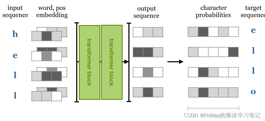
With RNNs this is all we need to do, since they cannot look forward into the input sequence: output i depends only on inputs 0 to i. With a transformer, the output depends on the entire input sequence, so prediction of the next character becomes vacuously easy, just retrieve it from the input.
对于 RNN，这就是我们需要做的就是，因为它们无法向前查看输入序列：输出 i 仅取决于输入 3 到 i 。使用变压器时，输出取决于整个输入序列，因此预测下一个字符变得非常容易，只需从输入中检索即可。

To use self-attention as an autoregressive model, we’ll need to ensure that it cannot look forward into the sequence. We do this by applying a mask to the matrix of dot products, before the softmax is applied. This mask disables all elements above the diagonal of the matrix.
要使用自我注意作为自回归模型，我们需要确保它不能向前看序列。为此，我们在应用 softmax 之前将掩码应用于点积矩阵。此掩码禁用矩阵对角线上方的所有元素。

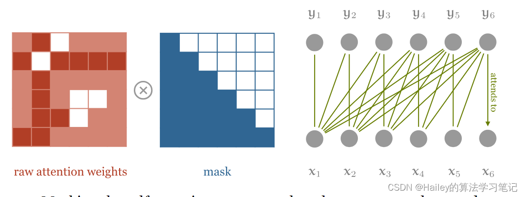
 Masking the self attention, to ensure that elements can only attend to input elements that precede them in the sequence. Note that the multiplication symbol is slightly misleading: we actually set the masked out elements (the white squares) to −∞
屏蔽自我注意，以确保元素只能关注序列中它们前面的输入元素。请注意，乘法符号略有误导：我们实际上将屏蔽的元素（白色方块）设置为 −∞

Since we want these elements to be zero after the softmax, we set them to −∞. Here’s how that looks in pytorch:
由于我们希望这些元素在softmax之后为零，因此我们将它们设置为 −∞ 。这是在pytorch中的样子：

dot = torch.bmm(queries, keys.transpose(1, 2))

indices = torch.triu_indices(t, t, offset=1)
dot[:, indices[0], indices[1]] = float('-inf')

dot = F.softmax(dot, dim=2)

After we’ve handicapped the self-attention module like this, the model can no longer look forward in the sequence.
在我们像这样阻碍了自我注意模块之后，模型就不能再在序列中向前看了。

We train on the standard enwik8 dataset (taken from the Hutter prize), which contains 108 characters of Wikipedia text (including markup). During training, we generate batches by randomly sampling subsequences from the data.
我们使用标准的 enwik8 数据集（取自 Hutter 奖）进行训练，其中包含 108 个字符的维基百科文本（包括标记）。在训练期间，我们通过从数据中随机采样子序列来生成批次。

We train on sequences of length 256, using a model of 12 transformer blocks and 256 embedding dimension. After about 24 hours training on an RTX 2080Ti (some 170K batches of size 32), we let the model generate from a 256-character seed: for each character, we feed it the preceding 256 characters, and look what it predicts for the next character (the last output vector). We sample from that with a temperature of 0.5, and move to the next character.
我们使用 12 个变压器块和 256 个嵌入维度的模型对长度为 256 的序列进行训练。在RTX 2080Ti（大约170K批次，大小为32）上训练大约24小时后，我们让模型从256个字符的种子生成：对于每个字符，我们向它输入前面的256个字符，并查看它对下一个字符（最后一个输出向量）的预测。我们从温度为 0.5 的那个位置采样，然后移动到下一个字符。

The output looks like this:
输出如下所示：

1228X Human & Rousseau. Because many of his stories were originally published in long-forgotten magazines and journals, there are a number of [[anthology|anthologies]] by different collators each containing a different selection. His original books have been considered an anthologie in the [[Middle Ages]], and were likely to be one of the most common in the [[Indian Ocean]] in the [[1st century]]. As a result of his death, the Bible was recognised as a counter-attack by the [[Gospel of Matthew]] (1177-1133), and the [[Saxony|Saxons]] of the [[Isle of Matthew]] (1100-1138), the third was a topic of the [[Saxony|Saxon]] throne, and the [[Roman Empire|Roman]] troops of [[Antiochia]] (1145-1148). The [[Roman Empire|Romans]] resigned in [[1148]] and [[1148]] began to collapse. The [[Saxony|Saxons]] of the [[Battle of Valasander]] reported the y
1228X 人类和卢梭。由于他的许多故事最初发表在早已被遗忘的杂志和期刊上，因此有许多由不同整理者撰写的[[选集|选集]]，每个选集都包含不同的选择。他的原著在[[中世纪]]被认为是选集，并且很可能是[[1世纪]][[印度洋]]最常见的作品之一。由于他的死，圣经被[[马太福音]]（1177-1133）和[[萨克森|撒克逊人]]的[[马修岛]]（1100-1138），第三个是[[萨克森|撒克逊]]的王位，以及[[罗马帝国|[[安条克]]（1145-1148）的罗马]军队。[[罗马帝国|罗马人]]在[[1148]]辞职，[[1148]]开始崩溃。[[萨克森|撒克逊人]]的[[瓦拉桑德战役]]报告了

Note that the Wikipedia link tag syntax is correctly used, that the text inside the links represents reasonable subjects for links. Most importantly, note that there is a rough thematic consistency; the generated text keeps on the subject of the bible, and the Roman empire, using different related terms at different points. While this is far from the performance of a model like GPT-2, the benefits over a similar RNN model are clear already: faster training (a similar RNN model would take many days to train) and better long-term coherence.
请注意，维基百科链接标签语法使用正确，链接中的文本表示链接的合理主题。最重要的是，请注意，有一个粗略的主题一致性;生成的文本继续围绕圣经和罗马帝国的主题，在不同的点上使用不同的相关术语。虽然这与 GPT-2 等模型的性能相去甚远，但与类似的 RNN 模型相比，它的好处已经很明显：更快的训练（类似的 RNN 模型需要很多天才能训练）和更好的长期连贯性。

In case you're curious, the Battle of Valasander seems to be an invention of the network.
如果你好奇，瓦拉桑德战役似乎是网络的发明。

At this point, the model achieves a compression of 1.343 bits per byte on the validation set, which is not too far off the state of the art of 0.93 bits per byte, achieved by the GPT-2 model (described below).
此时，该模型在验证集上实现了每字节 1.343 位的压缩，这与 GPT-2 模型（如下所述）实现的每字节 0.93 位的最新技术相差不远。

Design considerations 设计注意事项

To understand why transformers are set up this way, it helps to understand the basic design considerations that went into them. The main point of the transformer was to overcome the problems of the previous state-of-the-art architecture, the RNN (usually an LSTM or a GRU). Unrolled, an RNN looks like this:
要理解为什么以这种方式设置变压器，有助于理解其中的基本设计考虑因素。变压器的要点是克服以前最先进的架构RNN（通常是LSTM或GRU）的问题。展开后，RNN 如下所示：

 

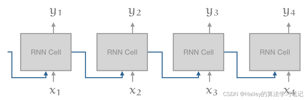
The big weakness here is the recurrent connection. while this allows information to propagate along the sequence, it also means that we cannot compute the cell at time step i until we’ve computed the cell at timestep i−1. Contrast this with a 1D convolution:
这里最大的弱点是反复连接。虽然这允许信息沿序列传播，但这也意味着我们无法在时间步长 i 计算单元格，直到我们在时间步长 2 i−1 计算单元格。将其与一维卷积进行对比：

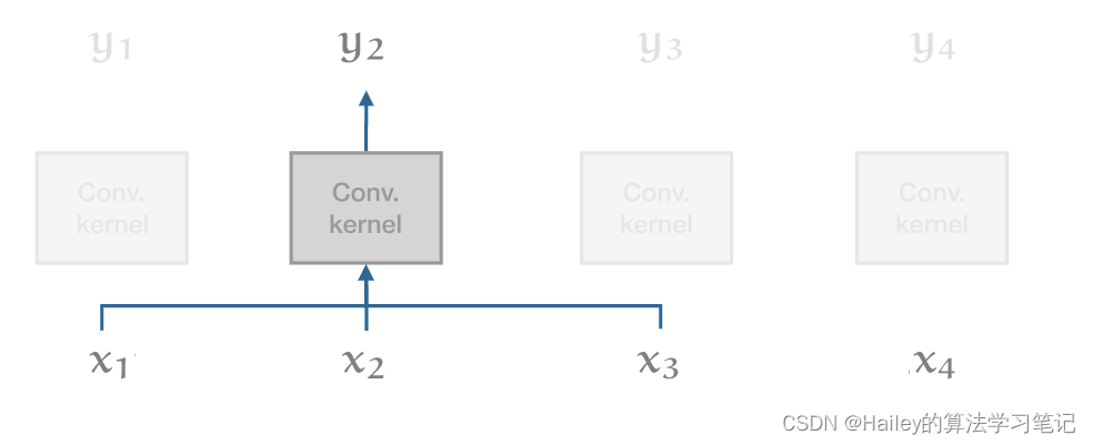
 In this model, every output vector can be computed in parallel with every other output vector. This makes convolutions much faster. The drawback with convolutions, however, is that they’re severely limited in modeling long range dependencies. In one convolution layer, only words that are closer together than the kernel size can interact with each other. For longer dependence we need to stack many convolutions.
在此模型中，每个输出向量都可以与其他每个输出向量并行计算。这使得卷积更快。然而，卷积的缺点是它们在对长程依赖关系进行建模时受到严重限制。在一个卷积层中，只有比内核大小更靠近的单词才能相互交互。对于更长的依赖性，我们需要堆叠许多卷积。

The transformer is an attempt to capture the best of both worlds. They can model dependencies over the whole range of the input sequence just as easily as they can for words that are next to each other (in fact, without the position vectors, they can’t even tell the difference). And yet, there are no recurrent connections, so the whole model can be computed in a very efficient feedforward fashion.
变压器试图捕捉两全其美。他们可以像对彼此相邻的单词一样轻松地对输入序列的整个范围内的依赖关系进行建模（事实上，如果没有位置向量，他们甚至无法区分）。然而，没有循环连接，因此可以以非常有效的前馈方式计算整个模型。

The rest of the design of the transformer is based primarily on one consideration: depth. Most choices follow from the desire to train big stacks of transformer blocks. Note for instance that there are only two places in the transformer where non-linearities occur: the softmax in the self-attention and the ReLU in the feedforward layer. The rest of the model is entirely composed of linear transformations, which perfectly preserve the gradient.
变压器的其余设计主要基于一个考虑因素：深度。大多数选择都是出于训练大堆变压器块的愿望。例如，请注意，变压器中只有两个地方出现非线性：自注意层中的softmax和前馈层中的ReLU。模型的其余部分完全由线性变换组成，完美地保留了梯度。

I suppose the layer normalization is also nonlinear, but that is one nonlinearity that actually helps to keep the gradient stable as it propagates back down the network.
我想层归一化也是非线性的，但这是一种非线性，实际上有助于保持梯度稳定，因为它沿着网络传播回去。

Historical baggage 历史包袱

If you’ve read other introductions to transformers, you may have noticed that they contain some bits I’ve skipped. I think these are not necessary to understand modern transformers. They are, however, helpful to understand some of the terminology and some of the writing about modern transformers. Here are the most important ones.
如果你读过其他关于变压器的介绍，你可能已经注意到它们包含了一些我跳过的部分。我认为这些对于了解现代变压器不是必需的。然而，它们有助于理解一些术语和一些关于现代变压器的文章。以下是最重要的。

Why is it called self-attention?
为什么叫自我注意？

Before self-attention was first presented, sequence models consisted mostly of recurrent networks or convolutions stacked together. At some point, it was discovered that these models could be helped by adding attention mechanisms: instead of feeding the output sequence of the previous layer directly to the input of the next, an intermediate mechanism was introduced, that decided which elements of the input were relevant for a particular word of the output.
在自我注意首次出现之前，序列模型主要由递归网络或堆叠在一起的卷积组成。在某些时候，人们发现这些模型可以通过添加注意力机制来帮助：不是将前一层的输出序列直接馈送到下一层的输入，而是引入了一种中间机制，该机制决定输入的哪些元素与输出的特定单词相关。

The general mechanism was as follows. We call the input the values. Some (trainable) mechanism assigns a key to each value. Then to each output, some other mechanism assigns a query.
总机制如下。我们将输入称为值。某些（可训练的）机制为每个值分配一个键。然后，对于每个输出，其他一些机制会分配一个查询。

These names derive from the datastructure of a key-value store. In that case we expect only one item in our store to have a key that matches the query, which is returned when the query is executed. Attention is a softened version of this: every key in the store matches the query to some extent. All are returned, and we take a sum, weighted by the extent to which each key matches the query.
这些名称派生自键值存储的数据结构。在这种情况下，我们希望商店中只有一个项目具有与查询匹配的键，该键在执行查询时返回。注意是软化版本：存储中的每个键都在某种程度上与查询匹配。所有内容都返回，我们取一个总和，按每个键与查询匹配的程度进行加权。

The great breakthrough of self-attention was that attention by itself is a strong enough mechanism to do all the learning. Attention is all you need, as the authors put it. The key, query and value are all the same vectors (with minor linear transformations). They attend to themselves and stacking such self-attention provides sufficient nonlinearity and representational power to learn very complicated functions.
自我注意的伟大突破在于，注意力本身就是一种足够强大的机制，可以完成所有的学习。正如作者所说，注意力就是你所需要的。键、查询和值都是相同的向量（具有较小的线性变换）。他们关注自己，堆叠这种自我注意力提供了足够的非线性和表征能力来学习非常复杂的函数。

The original transformer: encoders and decoders
原始变压器：编码器和解码器

But the authors did not dispense with all the complexity of contemporary sequence modeling. The standard structure of sequence-to-sequence models in those days was an encoder-decoder architecture, with teacher forcing.
但作者并没有放弃当代序列建模的所有复杂性。当时序列到序列模型的标准结构是编码器-解码器架构，带有教师强迫。

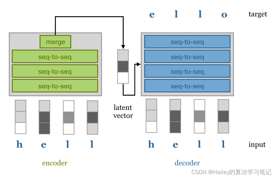
 The encoder takes the input sequence and maps it to a latent representation of the whole sequence. This can be either a sequence of latent vectors, or a single one as in the image above. This vector is then passed to a decoder which unpacks it to the desired target sequence (for instance, the same sentence in another language).
编码器获取输入序列并将其映射到整个序列的潜在表示形式。这可以是一系列潜在向量，也可以是上图所示的单个向量。然后将该向量传递给解码器，解码器将其解压缩为所需的目标序列（例如，另一种语言中的相同句子）。

Teacher forcing refers to the technique of also allowing the decoder access to the input sentence, but in an autoregressive fashion. That is, the decoder generates the output sentence word for word based both on the latent vector and the words it has already generated. This takes some of the pressure off the latent representation: the decoder can use word-for-word sampling to take care of the low-level structure like syntax and grammar and use the latent vector to capture more high-level semantic structure. Decoding twice with the same latent representation would, ideally, give you two different sentences with the same meaning.
教师强制是指也允许解码器访问输入句子的技术，但以自回归的方式。也就是说，解码器根据潜在向量和它已经生成的单词逐字生成输出句子。这减轻了潜在表示的一些压力：解码器可以使用逐字采样来处理语法和语法等低级结构，并使用潜在向量捕获更高级的语义结构。理想情况下，使用相同的潜在表示解码两次会给你两个具有相同含义的不同句子。

In later transformers, like BERT and GPT-2, the encoder/decoder configuration was entirely dispensed with. A simple stack of transformer blocks was found to be sufficient to achieve state of the art in many sequence based tasks.
在后来的变压器中，如BERT和GPT-2，编码器/解码器配置完全被省略了。发现一个简单的变压器块堆栈足以在许多基于序列的任务中实现最先进的技术。

This approach is sometimes called a decoder-only transformer (for an autoregressive model) or an encoder-only transformer (for a model without masking).
此方法有时称为仅解码器转换器（对于自回归模型）或仅编码器转换器（对于没有屏蔽的模型）。

Modern transformers 现代变压器

Here’s a small selection of some modern transformers and their most characteristic details.
以下是一些现代变压器的一小部分及其最具特色的细节。

BERT 伯特

BERT was one of the first models to show that transformers could reach human-level performance on a variety of language based tasks: question answering, sentiment classification or classifying whether two sentences naturally follow one another.
BERT是最早表明变形金刚可以在各种基于语言的任务上达到人类水平表现的模型之一：问答，情感分类或分类两个句子是否自然地相互跟随。

BERT consists of a simple stack of transformer blocks, of the type we’ve described above. This stack is pre-trained on a large general-domain corpus consisting of 800M words from English books (modern work, from unpublished authors), and 2.5B words of text from English Wikipedia articles (without markup).
BERT由一个简单的变压器块堆栈组成，我们上面描述的类型。该堆栈是在大型通用域语料库上进行预训练的，该语料库由来自英语书籍（现代作品，来自未出版作者）的 800M 个单词和来自英语维基百科文章的 2.5B 个单词的文本（没有标记）组成。

Pretraining is done through two tasks:
预训练通过两个任务完成：

Masking 掩蔽

A certain number of words in the input sequence are: masked out, replaced with a random word or kept as is. The model is then asked to predict, for these words, what the original words were. Note that the model doesn't need to predict the entire denoised sentence, just the modified words. Since the model doesn't know which words it will be asked about, it learns a representation for every word in the sequence.
输入序列中一定数量的单词是：屏蔽掉、替换为随机单词或保持原样。然后要求模型预测这些单词的原始单词是什么。请注意，该模型不需要预测整个去噪句子，只需要预测修改后的单词。由于模型不知道会询问哪些单词，因此它会学习序列中每个单词的表示形式。

Next sequence classification
下一个序列分类

Two sequences of about 256 words are sampled that either (a) follow each other directly in the corpus, or (b) are both taken from random places. The model must then predict whether a or b is the case.
对两个大约 256 个单词的序列进行采样，要么 （a） 直接在语料库中相互跟随，要么 （b） 都取自随机位置。然后，模型必须预测是 a 还是 b。

BERT uses WordPiece tokenization, which is somewhere in between word-level and character level sequences. It breaks words like walking up into the tokens walk and ##ing. This allows the model to make some inferences based on word structure: two verbs ending in -ing have similar grammatical functions, and two verbs starting with walk- have similar semantic function.
BERT使用WordPiece标记化，它介于单词级别和字符级别序列之间。它打破了诸如走进令牌步行和##ing之类的词。这允许模型根据单词结构进行一些推断：两个以-ing结尾的动词具有相似的语法功能，两个以walk-开头的动词具有相似的语义功能。

The input is prepended with a special <cls> token. The output vector corresponding to this token is used as a sentence representation in sequence classification tasks like the next sentence classification (as opposed to the global average pooling over all vectors that we used in our classification model above).
输入前面有一个特殊标记。对应于此标记的输出向量在序列分类任务（如下一个句子分类）中用作句子表示（与我们上面分类模型中使用的所有向量的全局平均池相反）。

After pretraining, a single task-specific layer is placed after the body of transformer blocks, which maps the general purpose representation to a task specific output. For classification tasks, this simply maps the first output token to softmax probabilities over the classes. For more complex tasks, a final sequence-to-sequence layer is designed specifically for the task.
预训练后，在转换器块主体之后放置一个特定于任务的层，该层将通用表示映射到特定于任务的输出。对于分类任务，这只是将第一个输出标记映射到类上的 softmax 概率。对于更复杂的任务，最终的序列到序列层是专门为该任务设计的。

The whole model is then re-trained to finetune the model for the specific task at hand.
然后重新训练整个模型，以针对手头的特定任务微调模型。

In an ablation experiment, the authors show that the largest improvement as compared to previous models comes from the bidirectional nature of BERT. That is, previous models like GPT used an autoregressive mask, which allowed attention only over previous tokens. The fact that in BERT all attention is over the whole sequence is the main cause of the improved performance.
在消融实验中，作者表明，与以前的模型相比，最大的改进来自BERT的双向性质。也就是说，像 GPT 这样的以前的模型使用自回归掩码，它只允许关注以前的令牌。在BERT中，所有注意力都集中在整个序列上，这是性能提高的主要原因。

This is why the B in BERT stands for "bidirectional".
这就是为什么BERT中的B代表“双向”。

The largest BERT model uses 24 transformer blocks, an embedding dimension of 1024 and 16 attention heads, resulting in 340M parameters.
最大的BERT模型使用24个变压器块，嵌入尺寸为1024和16个注意头，产生340M参数。

GPT-2 GPT-2

GPT-2 is the first transformer model that actually made it into the mainstream news, after the controversial decision by OpenAI not to release the full model.
GPT-2 是第一个真正成为主流新闻的变压器模型，此前 OpenAI 决定不发布完整模型。

The reason was that GPT-2 could generate sufficiently believable text that large-scale fake news campaigns of the kind seen in the 2016 US presidential election would become effectively a one-person job.
原因是 GPT-2 可以生成足够可信的文本，以至于 2016 年美国总统大选中看到的那种大规模假新闻活动实际上将成为一个人的工作。

The first trick that the authors of GPT-2 employed was to create a new high-quality dataset. While BERT used high-quality data, their sources (lovingly crafted books and well-edited wikipedia articles) had a certain lack of diversity in the writing style. To collect more diverse data without sacrificing quality the authors used links posted on the social media site Reddit to gather a large collection of writing with a certain minimum level of social support (expressed on Reddit as karma).
GPT-2 的作者采用的第一个技巧是创建一个新的高质量数据集。虽然BERT使用了高质量的数据，但他们的来源（精心制作的书籍和精心编辑的维基百科文章）在写作风格上缺乏多样性。为了在不牺牲质量的情况下收集更多样化的数据，作者使用社交媒体网站Reddit上发布的链接来收集大量具有一定最低社会支持水平的文章（在Reddit上表示为业力）。

GPT2 is fundamentally a language generation model, so it uses masked self-attention like we did in our model above. It uses byte-pair encoding to tokenize the language, which , like the WordPiece encoding breaks words up into tokens that are slightly larger than single characters but less than entire words.
GPT2 基本上是一个语言生成模型，因此它使用屏蔽的自我注意，就像我们在上面的模型中所做的那样。它使用字节对编码来标记语言，就像WordPiece编码一样，将单词分解为比单个字符略大但小于整个单词的标记。

GPT2 is built very much like our text generation model above, with only small differences in layer order and added tricks to train at greater depths. The largest model uses 48 transformer blocks, a sequence length of 1024 and an embedding dimension of 1600, resulting in 1.5B parameters.
GPT2 的构建方式非常类似于我们上面的文本生成模型，在层顺序上只有很小的差异，并添加了在更深深度进行训练的技巧。最大的模型使用 48 个变压器块，序列长度为 1024，嵌入维度为 1600，从而产生 1.5B 参数。

They show state-of-the art performance on many tasks. On the wikipedia compression task that we tried above, they achieve 0.93 bits per byte.
它们在许多任务上表现出最先进的性能。在我们上面尝试的维基百科压缩任务中，它们实现了每字节 0.93 位。

Transformer-XL 变压器-XL

While the transformer represents a massive leap forward in modeling long-range dependency, the models we have seen so far are still fundamentally limited by the size of the input. Since the size of the dot-product matrix grows quadratically in the sequence length, this quickly becomes the bottleneck as we try to extend the length of the input sequence. Transformer-XL is one of the first succesful transformer models to tackle this problem.
虽然变压器代表了长期依赖性建模的巨大飞跃，但到目前为止我们看到的模型仍然从根本上受到输入大小的限制。由于点积矩阵的大小在序列长度中呈二次增长，因此当我们尝试扩展输入序列的长度时，这很快就会成为瓶颈。Transformer-XL是最早成功解决此问题的变压器型号之一。

During training, a long sequence of text (longer than the model could deal with) is broken up into shorter segments. Each segment is processed in sequence, with self-attention computed over the tokens in the curent segment and the previous segment. Gradients are only computed over the current segment, but information still propagates as the segment window moves through the text. In theory at layer n, information may be used from n segments ago.
在训练期间，一长串文本（比模型可以处理的长）被分解成较短的片段。每个段都按顺序处理，对当前段和前一个段中的标记计算自我注意。梯度仅在当前句段上计算，但信息仍会随着句段窗口在文本中的移动而传播。理论上在第 层 1 处，可以使用从 n 段前的信息。

A similar trick in RNN training is called truncated backpropagation through time. We feed the model a very long sequence, but backpropagate only over part of it. The first part of the sequence, for which no gradients are computed, still influences the values of the hidden states in the part for which they are.
RNN 训练中的类似技巧称为截断反向传播随时间变化。我们为模型提供很长的序列，但只在部分序列上反向传播。序列的第一部分（不计算梯度）仍然影响隐藏状态所在部分中隐藏状态的值。

To make this work, the authors had to let go of the standard position encoding/embedding scheme. Since the position encoding is absolute, it would change for each segment and not lead to a consistent embedding over the whole sequence. Instead they use a relative encoding. For each output vector, a different sequence of position vectors is used that denotes not the absolute position, but the distance to the current output.
为了完成这项工作，作者不得不放弃标准的位置编码/嵌入方案。由于位置编码是绝对的，因此每个段都会发生变化，并且不会导致整个序列的一致嵌入。相反，它们使用相对编码。对于每个输出向量，使用不同的位置向量序列，该向量不表示绝对位置，而是表示到当前输出的距离。

This requires moving the position encoding into the attention mechanism (which is detailed in the paper). One benefit is that the resulting transformer will likely generalize much better to sequences of unseen length.
这需要将位置编码移动到注意力机制中（本文对此进行了详细说明）。一个好处是，由此产生的变压器可能会更好地推广到看不见的长度序列。

Sparse transformers 稀疏变压器

Sparse transformers tackle the problem of quadratic memory use head-on. Instead of computing a dense matrix of attention weights (which grows quadratically), they compute the self-attention only for particular pairs of input tokens, resulting in a sparse attention matrix, with only nn−−√ explicit elements.
稀疏变压器正面解决了二次存储器使用的问题。他们没有计算注意力权重的密集矩阵（二次增长），而是仅计算特定输入令牌对的自我注意，从而产生一个稀疏的注意力矩阵，只有 nn−−√ 个显式元素。

This allows models with very large context sizes, for instance for generative modeling over images, with large dependencies between pixels. The tradeoff is that the sparsity structure is not learned, so by the choice of sparse matrix, we are disabling some interactions between input tokens that might otherwise have been useful. However, two units that are not directly related may still interact in higher layers of the transformer (similar to the way a convolutional net builds up a larger receptive field with more convolutional layers).
这允许具有非常大的上下文大小的模型，例如用于图像的生成建模，像素之间具有很大的依赖关系。权衡是没有学习稀疏性结构，因此通过选择稀疏矩阵，我们正在禁用输入令牌之间的一些交互，否则这些交互可能很有用。然而，两个没有直接关系的单元可能仍然在变压器的更高层中相互作用（类似于卷积网络建立具有更多卷积层的更大感受野的方式）。

Beyond the simple benefit of training transformers with very large sequence lengths, the sparse transformer also allows a very elegant way of designing an inductive bias. We take our input as a collection of units (words, characters, pixels in an image, nodes in a graph) and we specify, through the sparsity of the attention matrix, which units we believe to be related. The rest is just a matter of building the transformer up as deep as it will go and seeing if it trains.
除了训练具有非常大序列长度的变压器的简单好处之外，稀疏变压器还允许以非常优雅的方式设计电感偏置。我们将输入作为单位（单词，字符，图像中的像素，图形中的节点）的集合，并通过注意力矩阵的稀疏性指定我们认为哪些单位是相关的。剩下的只是将变压器建造得尽可能深，看看它是否训练。

Going big 做大

The big bottleneck in training transformers is the matrix of dot products in the self attention. For a sequence length t, this is a dense matrix containing t2 elements. At standard 32-bit precision, and with t=1000 a batch of 16 such matrices takes up about 250Mb of memory. Since we need at least four of them per self attention operation (before and after softmax, plus their gradients), that limits us to at most twelve layers in a standard 12Gb GPU. In practice, we get even less, since the inputs and outputs also take up a lot of memory (although the dot product dominates).
训练变压器的最大瓶颈是自我注意力中的点积矩阵。对于序列长度 t ，这是一个包含 t2 个元素的密集矩阵。在标准的 32 位精度下，对于 t=1000 ，一批 16 个这样的矩阵占用大约 250Mb 的内存。由于我们每个自我注意操作至少需要四个（在softmax之前和之后，加上它们的梯度），这限制了我们在标准12GbGPU中最多十二层。在实践中，我们得到的甚至更少，因为输入和输出也占用大量内存（尽管点积占主导地位）。

And yet models reported in the literature contain sequence lengths of over 12000, with 48 layers, using dense dot product matrices. These models are trained on clusters, of course, but a single GPU is still required to do a single forward/backward pass. How do we fit such humongous transformers into 12Gb of memory? There are three main tricks:
然而，文献中报道的模型包含超过12000的序列长度，有48层，使用密集的点积矩阵。当然，这些模型是在集群上训练的，但仍然需要一个 GPU 来执行一次前进/后退传递。我们如何将如此巨大的变压器安装到 12Gb 的内存中？有三个主要技巧：

Half precision 半精度

On modern GPUs and on TPUs, tensor computations can be done efficiently on 16-bit float tensors. This isn't quite as simple as just setting the dtype of the tensor to torch.float16. For some parts of the network, like the loss, 32 bit precision is required. But most of this can be handled with relative ease by existing libraries. Practically, this doubles your effective memory.
在现代 GPU 和 TPU 上，张量计算可以在 16 位浮点张量上高效完成。这并不像将张量的 dtype 设置为 torch.float16 那么简单。对于网络的某些部分，如损耗，需要32位精度。但其中大部分都可以由现有库相对轻松地处理。实际上，这会使您的有效内存翻倍。

Gradient accumulation 梯度累积

For a large model, we may only be able to perform a forward/backward pass on a single instance. Batch size 1 is not likely to lead to stable learning. Luckily, we can perform a single forward/backward for each instance in a larger batch, and simply sum the gradients we find (this is a consequence of the multivariate chain rule). When we hit the end of the batch, we do a single step of gradient descent, and zero out the gradient. In Pytorch this is particulary easy: you know that optimizer.zero_grad() call in your training loop that seems so superfluous? If you don't make that call, the new gradients are simply added to the old ones.
对于大型模型，我们可能只能在单个实例上执行向前/向后传递。批量大小 1 不太可能导致稳定的学习。幸运的是，我们可以在更大的批次中为每个实例执行单个向前/向后执行一次，并简单地对我们发现的梯度求和（这是多元链规则的结果）。当我们到达批次的末尾时，我们执行梯度下降的单步，并将梯度归零。在 Pytorch 中，这特别容易：你知道训练循环中的 optimizer.zero_grad() 调用看起来如此多余吗？如果您不进行该调用，则只需将新渐变添加到旧梯度中。

Gradient checkpointing 渐变检查点

If your model is so big that even a single forward/backward won't fit in memory, you can trade off even more computation for memory efficiency. In gradient checkpointing, you separate your model into sections. For each section, you do a separate forward/backward to compute the gradients, without retaining the intermediate values for the rest. Pytorch has special utilities for gradient checkpointng.
如果您的模型太大，以至于即使是单个向前/向后也无法放入内存，则可以牺牲更多的计算来获得内存效率。在梯度检查点中，将模型分成多个部分。对于每个部分，您执行单独的前进/后退以计算梯度，而不保留其余部分的中间值。Pytorch具有用于梯度检查点的特殊实用程序。

For more information on how to do this, see this blogpost.
有关如何执行此操作的详细信息，请参阅此博客文章。

Conclusion 结论

The transformer may well be the simplest machine learning architecture to dominate the field in decades. There are good reasons to start paying attention to them if you haven’t been already.
转换器很可能是几十年来主导该领域的最简单的机器学习架构。如果你还没有去过，有充分的理由开始关注它们。

Firstly, the current performance limit is purely in the hardware. Unlike convolutions or LSTMs the current limitations to what they can do are entirely determined by how big a model we can fit in GPU memory and how much data we can push through it in a reasonable amount of time. I have no doubt, we will eventually hit the point where more layers and and more data won’t help anymore, but we don’t seem to have reached that point yet.
首先，当前的性能限制纯粹在硬件上。与卷积或 LSTM 不同，它们目前可以执行的操作限制完全取决于我们可以在 GPU 内存中容纳多大的模型以及我们可以在合理的时间内推送多少数据。我毫不怀疑，我们最终会达到更多的层和更多的数据将不再有帮助的地步，但我们似乎还没有达到这一点。

Second, transformers are extremely generic. So far, the big successes have been in language modelling, with some more modest achievements in image and music analysis, but the transformer has a level of generality that is waiting to be exploited. The basic transformer is a set-to-set model. So long as your data is a set of units, you can apply a transformer. Anything else you know about your data (like local structure) you can add by means of position embeddings, or by manipulating the structure of the attention matrix (making it sparse, or masking out parts).
其次，变压器非常通用。到目前为止，最大的成功是在语言建模方面，在图像和音乐分析方面取得了一些较为温和的成就，但转换器的通用性水平正在等待被利用。基本变压器是一组到设置的模型。只要您的数据是一组单位，就可以应用转换器。您知道的有关数据的任何其他信息（如局部结构）都可以通过位置嵌入或操作注意力矩阵的结构（使其稀疏或屏蔽部分）来添加。

This is particularly useful in multi-modal learning. We could easily combine a captioned image into a set of pixels and characters and design some clever embeddings and sparsity structure to help the model figure out how to combine and align the two. If we combine the entirety of our knowledge about our domain into a relational structure like a multi-modal knowledge graph (as discussed in [3]), simple transformer blocks could be employed to propagate information between multimodal units, and to align them with the sparsity structure providing control over which units directly interact.
这在多模态学习中特别有用。我们可以轻松地将带标题的图像组合成一组像素和字符，并设计一些巧妙的嵌入和稀疏结构，以帮助模型弄清楚如何组合和对齐两者。如果我们将关于我们领域的全部知识组合成一个关系结构，如多模态知识图谱（如[3]中所述），则可以使用简单的变压器块在多模态单元之间传播信息，并将它们与稀疏结构对齐，从而控制哪些单元直接交互。

So far, transformers are still primarily seen as a language model. I expect that in time, we’ll see them adopted much more in other domains, not just to increase performance, but to simplify existing models, and to allow practitioners more intuitive control over their models’ inductive biases.
到目前为止，变压器仍然主要被视为一种语言模型。我希望随着时间的推移，我们将看到它们在其他领域得到更多的采用，不仅仅是为了提高性能，而且是为了简化现有模型，并允许从业者更直观地控制他们模型的归纳偏差。

References 引用

[1] The illustrated transformer, Jay Allamar.
[1] 图解变形金刚，杰伊·阿拉马尔。

[2] The annotated transformer, Alexander Rush.
[2] 带注释的变压器，亚历山大·拉什。

[3] The knowledge graph as the default data model for learning on heterogeneous knowledge Xander Wilcke, Peter Bloem, Victor de Boer
[3] 知识图谱作为异构知识学习的默认数据模型 Xander Wilcke， Peter Bloem， Victor de Boer

[4] Matrix factorization techniques for recommender systems Yehuda Koren et al.
[4] 推荐系统的矩阵分解技术 Yehuda Koren et al.

Updates 更新

19 October 2019 19 十月 2019

Added a section on the difference between wide and narrow self-attention. Thanks to Sidney Melo for spotting the mistake in the original implementation.
增加了一个关于宽自我注意和狭义自我注意之间区别的部分。感谢 Sidney Melo 发现了原始实现中的错误。

9 December 2022 9 十二月 2022

Clarified the example in the section on multi-head attention.
澄清了多头注意力部分中的示例。

4 March 2023 4 三月 2023

Fixed a persistent mistake in the defintition of multi-head self-attention. Rewrote the final self-attention to be the canonical form (rather than the earlier "wide" variety we used for the sake of simplicity).
修复了多头自我注意定义中的一个持续错误。将最终的自我注意重写为规范形式（而不是我们为了简单起见而使用的早期“广泛”变体）。

BACK

TRANSFORMERS FROM SCRATCH