机器学习笔记--简单创建一个模型

引入包：

from learntools.core import binder
binder.bind(globals())
from learntools.machine_learning.ex2 import *

import pandas as pd

读取数据：

# Path of the file to read
iowa_file_path = '../input/home-data-for-ml-course/train.csv'

# Fill in the line below to read the file into a variable home_data
home_data = pd.read_csv(iowa_file_path)

home_data.columns     #返回所有列的列表

LotArea = home_data.loc[:,"LotArea"]   #读取表格中的一列数据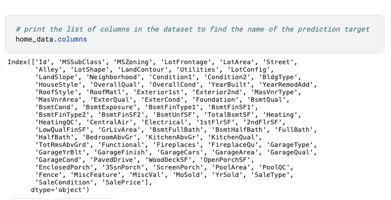

数据预处理：

（删除缺失值只是处理缺失值的方法之一）

home_data = home_data.dropna(axis=0)    #dropna()用于删除删除丢失的值，axis=0:按行删除；1:按列删除

缺失值处理方法：

1. 整列数据删除：

# 提取出含有缺失值的列
cols_with_missing = [col for col in X_train.columns
                     if X_train[col].isnull().any()]

# 在训练集和测试集中删除含有缺失值的列，得到新的训练集和测试集
reduced_X_train = X_train.drop(cols_with_missing, axis=1)
reduced_X_valid = X_valid.drop(cols_with_missing, axis=1)

1. 插补法（用这一列的平均值填充缺失值）：

from sklearn.impute import SimpleImputer

# 用数据的平均值填充缺失值，得到新的训练集和测试集
my_imputer = SimpleImputer()
imputed_X_train = pd.DataFrame(my_imputer.fit_transform(X_train))    #对X_train计算均值，然后把训练集的缺失值填充平均值
imputed_X_valid = pd.DataFrame(my_imputer.transform(X_valid)) #      对测试值的缺失值进行填充

# Imputation removed column names; put them back
imputed_X_train.columns = X_train.columns
imputed_X_valid.columns = X_valid.columns

处理分类变量的方法：

1. Drop Categorical Variables 不考虑分类变量对因变量的影响；

#把分类自变量直接剔除，得到新的训练集和测试集
drop_X_train = X_train.select_dtypes(exclude = ['object'])
drop_X_valid = X_valid.select_dtypes(exclude = ['object'])

1. Ordinal Encoding将分类变量转化成数值：

# Categorical columns in the training data
object_cols = [col for col in X_train.columns if X_train[col].dtype == "object"]

# Columns that can be safely ordinal encoded
good_label_cols = [col for col in object_cols if 
                   set(X_valid[col]).issubset(set(X_train[col]))]
        
# Problematic columns that will be dropped from the dataset
bad_label_cols = list(set(object_cols)-set(good_label_cols))
 
from sklearn.preprocessing import OrdinalEncoder

#找到训练集和测试集中文本格式的数据，将这些数据都删除
label_X_train = X_train.drop(bad_label_cols, axis=1)
label_X_valid = X_valid.drop(bad_label_cols, axis=1)

#对缺失值进行填充，得到新的测试集和训练集数据
ordinarial_encoder = OrdinalEncoder()
label_X_train[good_label_cols] = ordinarial_encoder.fit_transform(X_train[good_label_cols])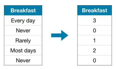
label_X_valid[good_label_cols] = ordinarial_encoder.transform(X_valid[good_label_cols])

1. One-Hot Encoding：

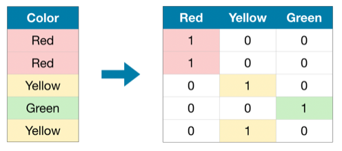
将一列颜色数据转化成红、黄、绿三列数据，“1”代表是，而“0”代表不是。

# Get number of unique entries in each column with categorical data
object_nunique = list(map(lambda col: X_train[col].nunique(), object_cols))
d = dict(zip(object_cols, object_nunique))

# 可以得到每一列的标题及每一列有几类文本
sorted(d.items(), key=lambda x: x[1])

#将分类变量区分为高类别变量与低类别变量
# 低类别变量可以用one-hot
low_cardinality_cols = [col for col in object_cols if X_train[col].nunique() < 10]

# 高类别变量将被剔除
high_cardinality_cols = list(set(object_cols)-set(low_cardinality_cols))

from sklearn.preprocessing import OneHotEncoder

# Apply one-hot encoder to each column with categorical data
OH_encoder = OneHotEncoder(handle_unknown='ignore', sparse=False)
OH_cols_train = pd.DataFrame(OH_encoder.fit_transform(X_train[low_cardinality_cols]))
OH_cols_valid = pd.DataFrame(OH_encoder.transform(X_valid[low_cardinality_cols]))

# One-hot encoding removed index; put it back
OH_cols_train.index = X_train.index
OH_cols_valid.index = X_valid.index

# Remove categorical columns (will replace with one-hot encoding)
num_X_train = X_train.drop(object_cols, axis=1)
num_X_valid = X_valid.drop(object_cols, axis=1)

# Add one-hot encoded columns to numerical features
OH_X_train = pd.concat([num_X_train, OH_cols_train], axis=1)
OH_X_valid = pd.concat([num_X_valid, OH_cols_valid], axis=1)

选择自变量：

构建一个只有几个特征作为自变量和因变量的模型：

y = home_data.SalePrice

# Create the list of features below
feature_names = ['LotArea','YearBuilt','1stFlrSF','2ndFlrSF','FullBath','BedroomAbvGr','TotRmsAbvGrd']

# Select data corresponding to features in feature_names
X = home_data[feature_names]

# Review data
# print description or statistics from X
print(X.describe())

# print the top few lines
print(X.head())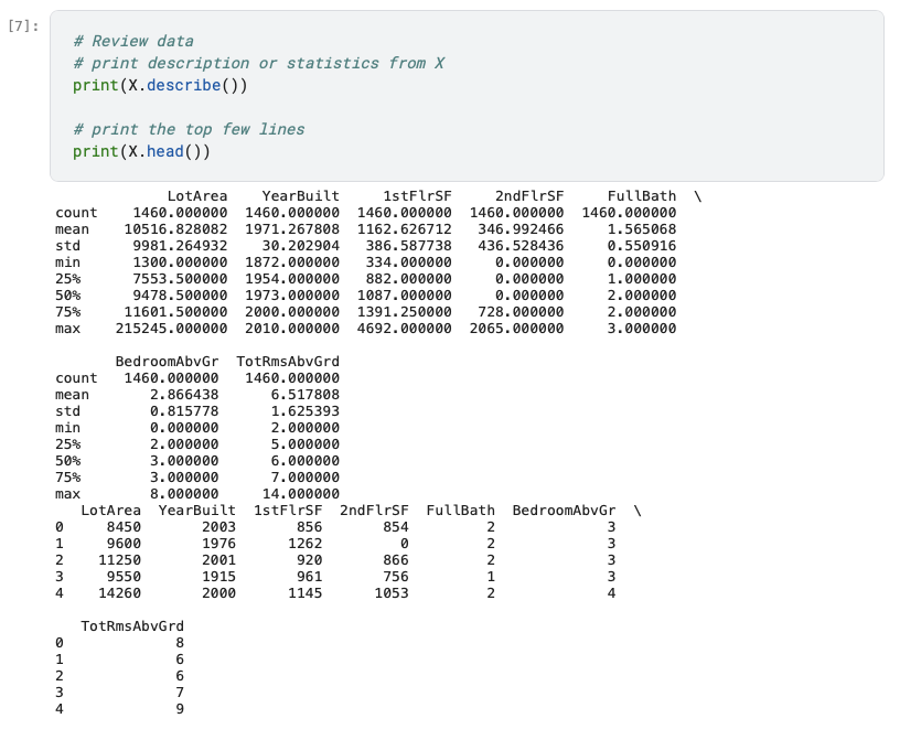

模型搭建、训练和测试：

#将数据集划分为训练集和测试集
from sklearn.model_selection import train_test_split
train_X, val_X, train_y, val_y = train_test_split(X,y,random_state=1)

决策树模型：

from sklearn.tree import DecisionTreeRegressor
#specify the model. 
#For model reproducibility, set a numeric value for random_state when specifying the model
iowa_model = DecisionTreeRegressor(random_state=1)

# Fit the model
iowa_model.fit(train_X,train_y)

#predict model
predictions = iowa_model.predict(val_X)

随机森林模型：

from sklearn.ensemble import RandomForestRegressor

forest_model = RandomForestRegressor(random_state=1)
forest_model.fit(train_X, train_y)
melb_preds = forest_model.predict(val_X)

计算误差：

模型的预测结果与实际值之间的平均绝对误差：

from sklearn.metrics import mean_absolute_error

predicted_home_prices = melbourne_model.predict(val_X)
mean_absolute_error(val_y, predicted_home_prices)      #计算模型的平均绝对误差   

欠拟合与过拟合：

欠拟合：模型无法捕捉数据中的重要区别和模式，因此即使在训练数据中也表现不佳；

过拟合：一个模型几乎完美地匹配训练数据，但在验证和其他新数据方面表现不佳。

通过控制模型的最大叶子数，逐个输出模型预测值与实际值平均绝对误差，进而比较模型在什么区间内过拟合，选择拟合效果最好的模型：

from sklearn.metrics import mean_absolute_error
from sklearn.tree import DecisionTreeRegressor

def get_mae(max_leaf_nodes, train_X, val_X, train_y, val_y):
    model = DecisionTreeRegressor(max_leaf_nodes=max_leaf_nodes, random_state=0)
    model.fit(train_X, train_y)
    preds_val = model.predict(val_X)
    mae = mean_absolute_error(val_y, preds_val)
    return(mae)

candidate_max_leaf_nodes = [5, 25, 50, 100, 250, 500]
# Write loop to find the ideal tree size from candidate_max_leaf_nodes
for max_leaf_nodes in candidate_max_leaf_nodes:
    my_mae = get_mae(max_leaf_nodes, train_X, val_X, train_y, val_y)
    print("Max leaf nodes: %d  \t\t Mean Absolute Error:  %d" %(max_leaf_nodes, my_mae))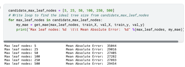

可以看到最大叶子结点数为100时，平均绝对误差最小。

best_tree_size = 100

# 建立新的决策树模型
final_model = DecisionTreeRegressor(max_leaf_nodes=best_tree_size, random_state=1)

# fit the final model and uncomment the next two lines
final_model.fit(X, y)

Pipelines：

流水线是将处理数据、搭建模型等代码组装在一起，在使用的时候更方便。

优点：

1. 代码更简洁；
2. 错误率更低；
3. 生产率更高；
4. 模型验证的更多选项。

步骤：

1. 定义预处理：

1） 在数值数据中输入缺失的值

2）输入缺失值并对分类数据应用one-hot编码

from sklearn.compose import ColumnTransformer
from sklearn.pipeline import Pipeline
from sklearn.impute import SimpleImputer
from sklearn.preprocessing import OneHotEncoder

# Preprocessing for numerical data
numerical_transformer = SimpleImputer(strategy='constant')

# Preprocessing for categorical data
categorical_transformer = Pipeline(steps=[
    ('imputer', SimpleImputer(strategy='most_frequent')),
    ('onehot', OneHotEncoder(handle_unknown='ignore'))
])

# Bundle preprocessing for numerical and categorical data
preprocessor = ColumnTransformer(
    transformers=[
        ('num', numerical_transformer, numerical_cols),
        ('cat', categorical_transformer, categorical_cols)
    ])

1. 定义模型：

from sklearn.ensemble import RandomForestRegressor

model = RandomForestRegressor(n_estimators=100, random_state=0)

1. 创建并评估流水线：

from sklearn.metrics import mean_absolute_error

# Bundle preprocessing and modeling code in a pipeline
my_pipeline = Pipeline(steps=[('preprocessor', preprocessor),
                              ('model', model)
                             ])

# Preprocessing of training data, fit model 
my_pipeline.fit(X_train, y_train)

# Preprocessing of validation data, get predictions
preds = my_pipeline.predict(X_valid)

# Evaluate the model
score = mean_absolute_error(y_valid, preds)
print('MAE:', score)

交叉验证：

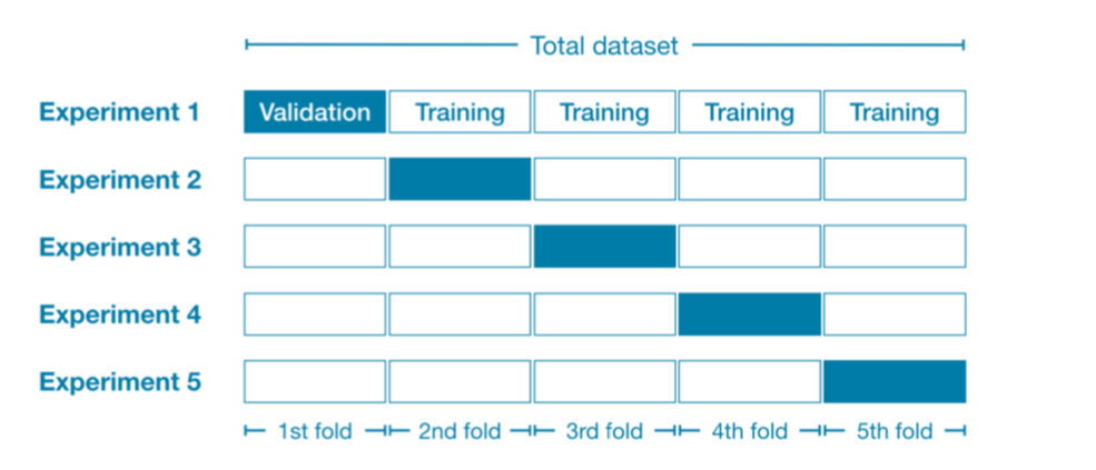
将数据分成5份，第一次把第一份数据集作为验证集，其余四份作为训练集，以此类推，共进行五次实验。

from sklearn.model_selection import cross_val_score

# Multiply by -1 since sklearn calculates *negative* MAE
scores = -1 * cross_val_score(my_pipeline, X, y,
                              cv=5,      #进行五次实验
                              scoring='neg_mean_absolute_error')

final_score = scores.mean()    #取平均

梯度增加：

步骤：

XGBoost是梯度增加的一个应用：

from xgboost import XGBRegressor

my_model = XGBRegressor()
my_model.fit(X_train, y_train)

XGBRegressor（）的参数：

n_estimators表示循环多少次：

my_model = XGBRegressor(n_estimators=500)   
my_model.fit(X_train, y_train)

learning_rate表示迭代决策树的步长，若learning_rate越小，则越有可能找到更精确的最佳值，但迭代速度也更慢:

my_model = XGBRegressor(n_estimators=1000, learning_rate=0.05)   
my_model.fit(X_train, y_train, 
             early_stopping_rounds=5, 
             eval_set=[(X_valid, y_valid)], 
             verbose=False)

n_jobs表示:

my_model = XGBRegressor(n_estimators=1000, learning_rate=0.05, n_jobs=4)
my_model.fit(X_train, y_train, 
             early_stopping_rounds=5, 
             eval_set=[(X_valid, y_valid)], 
             verbose=False)

my_model = XGBRegressor(n_estimators=500)
my_model.fit(X_train, y_train, 
             early_stopping_rounds=5,       #early_stopping_rounds设置最少循环的次数
             eval_set=[(X_valid, y_valid)],
             verbose=False)

数据泄漏：

数据泄露发生的情况一般是训练数据包含了因变量。数据泄漏的表现一般是训练的模型的准确率异常得好，但实际上预测的结果却很差

分类：

1. 目标数据泄露

在所给的数据中有两列数据含有强烈的相关性，虽然在实验数据中，可以得到很好的结果，但在现实生活中很难应用。

1. 训练测试数据泄漏

训练集和测试集数据划分的不准确性。

expenditures_cardholders = X.expenditure[y]
expenditures_noncardholders = X.expenditure[~y]

# 挑选出可能会造成数据泄漏的数据剔除
potential_leaks = ['expenditure', 'share', 'active', 'majorcards']
X2 = X.drop(potential_leaks, axis=1)

# Evaluate the model with leaky predictors removed
cv_scores = cross_val_score(my_pipeline, X2, y, 
                            cv=5,
                            scoring='accuracy')