


目录
0 概述:
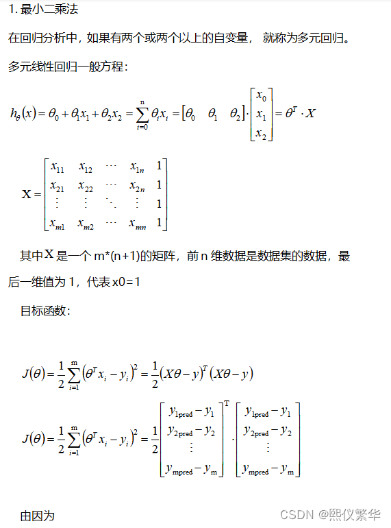
前面基于最小二乘法求解的思路是通过给出的样本直接求解析解:
那么有没有一种方法,首先先随便给出一条直线,让他慢慢拟合到最优解位置,有:梯度下降法。
我们的目标是让目标函数(误差平方和)最小。
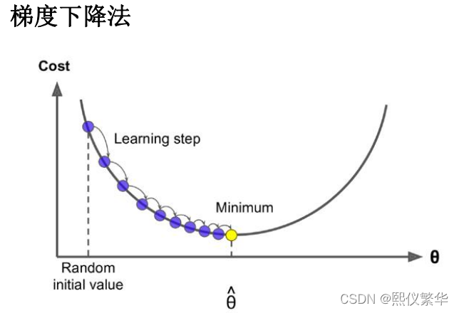
我们知道目标函数是一个凸函数,极值点,所以基本思想是,给出一个theta 不断调整theta的值,调整到让目标函数最小。
原因:
上面利用公式求解里面对称阵是N维乘以N维的,复 杂度是是O N的三次方,换句话说,就是如果你的特 征数量翻倍,你的计算时间大致上要2的三次方,8倍 的慢
Ø
梯度下降法(英语:
Gradient descent
)是一个 一阶最优化算法,通常也称为最速下降法。
Ø
梯度下降算法是一种求局部最优解的方法,对 于F(x)
,在
a
点的梯度是
F(x)
增长最快的方向,
那么它的相反方向则是该点下降最快的方向
Ø
原理:将函数比作一座山,站在某个山坡上,往四周看,从哪个方向向下走一小步,能够下
降的最快;
一 回顾最小二乘法


二 批量梯度下降法BGD


2.1自己推导理解xj:


2.2 批量梯度下降法BGD 代码实现:
import numpy as  np
x=np.array([4,8,5,10,12])
y=np.array([20,50,30,70,60])
# h_theta(x)=y=theta0+theta1*x
theta0,theta1=0,0
alpha=0.01
# 样本个数
m=len(x)
# 设置停止条件 计算mse的误差,如果误差小于等于epsilon 那么就停止
epsilon=0.00001
# 误差
error0,error1=0,0
# 计算迭代次数
cnt=0
def h_theta_x(x):
    return theta0+theta1*x
while True:
    cnt+=1
    diff=[0,0]  #初始化两个梯度
    for i in range(m):
        diff[0]+=(y[i]-h_theta_x(x[i]))*1
        diff[1] += (y[i] - h_theta_x(x[i])) * x[i]
    theta0=theta0+alpha*diff[0]/m
    theta1 = theta1 + alpha * diff[1]/m
    # 输出theta值
    print("theta0:%s,theta1:%s"%(theta0,theta1))
    # 计算mse
    for i in range(m):
        error1 +=(y[i]-h_theta_x(x[i]))**2
    error1/=m

    if(abs(error1-error0)<=epsilon):
        break
    else:
        error0=error1

print("迭代次数:%s"%cnt)
上述方式总结发现其实可以用矩阵表示:直接求所有梯度。
m个样本 有两个特征,根据特征求2个theta =【 theta0 theta1 】。
对theta0 求偏导时,
heta0 的偏导:theta0的特征x0有m个,为x01...... x0m 均为1;
heta1的偏导:theta1的特征x1有m个,为x11...... x1m;
2.3批量梯度下降法BGD 向量实现方式

import numpy as  np
x=np.array([[1,4],[1,8],[1,5],[1,10],[1,12]])
y=np.array([[20],[50],[30],[70],[60]])

x_b=x
m=len(y)
#最大迭代次数
n_iterations=10000
learn_rate=0.001
# 1,初始化theta,w0...wn
theta=np.random.randn(2,1)
# 2,不会设置阈值,直接设置超参数,迭代次数,迭代次数到了,我们就认为收敛了
for _ in range(n_iterations):
    # 3,接着求梯度gradient
    gradients=1/m*x_b.T.dot(x_b.dot(theta)-y)
    # 4,应用公式调整theta值,theta_t + 1 = theta_t - grad * learning_rate
    theta=theta-learn_rate*gradients
print(theta)
[[1.10392478]
[5.75063029]]

三 随机梯度下降SGD


3.1 随机梯度下降SGD 代码实现
import numpy as  np
x=np.array([4,8,5,10,12])
y=np.array([20,50,30,70,60])
# h_theta(x)=y=theta0+theta1*x
theta0,theta1=0,0
alpha=0.01
# 样本个数
m=len(x)
# 设置停止条件 计算mse的误差,如果误差小于等于epsilon 那么就停止
epsilon=0.00001
# 误差
error0,error1=0,0
# 计算迭代次数
cnt=0
def h_theta_x(x):
    return theta0+theta1*x
while True:
    cnt+=1
    diff=[0,0]  #初始化两个梯度
    i=np.random.randint(0,m)
    diff0=(y[i]-h_theta_x(x[i]))*1
    diff1=(y[i] - h_theta_x(x[i])) * x[i]
    theta0=theta0+alpha*diff0
    theta1 = theta1 + alpha * diff1
    # 输出theta值
    print("theta0:%s,theta1:%s"%(theta0,theta1))
    # 计算mse
    for i in range(m):
        error1 +=(y[i]-h_theta_x(x[i]))**2
    error1/=m

    if(abs(error1-error0)<=epsilon):
        break
    else:
        error0=error1

print("迭代次数:%s"%cnt)
3.2 SGD 向量形式:
import numpy as np

np.random.seed(1)
X = 2 * np.random.rand(100, 1)
y = 4 + 3 * X + np.random.randn(100, 1)
X_b = np.c_[np.ones((100, 1)), X]
# X_b = np.array([[1,4],[1,8],[1,5],[1,10],[1,12]])
# y = np.array([[20],[50],[30],[70],[60]])
# print(X_b)

learning_rate = 0.001
#最大迭代次数
n_iterations = 100000
m = len(y)
# 1,初始化theta,w0...wn
# theta = np.random.randn(2, 1)
theta = np.zeros((2,1))
# 4,不会设置阈值,直接设置超参数,迭代次数,迭代次数到了,我们就认为收敛了
for _ in range(n_iterations):
    # 2,接着求梯度gradient
    i=np.random.randint(0,m)
    X=X_b[i:i+1,:]
    gradients = X.T.dot(X.dot(theta)-y[i])
    # 3,应用公式调整theta值,theta_t + 1 = theta_t - grad * learning_rate
    theta = theta - learning_rate * gradients

print(theta)
3.3 SGD 动态改变学习率;
#!/usr/bin/python
# -*- coding: UTF-8 -*-
# 文件名: stochastic_gradient_descent1.py

import numpy as np


np.random.seed(1)
X = 2 * np.random.rand(100, 1)
y = 4 + 3 * X + np.random.randn(100, 1)
X_b = np.c_[np.ones((100, 1)), X]

n_epochs = 10000
t0, t1 = 5, 500  # 超参数

m = 100

def learning_schedule(t):
    return t0 / (t + t1)


# 1, 随机初始化
theta = np.random.randn(2, 1)


for epoch in range(n_epochs):
    for i in range(m):
        # 2, 求gradient Xi.T * (Xi * theta - yi)
        #随机取出一个样本和样本所对应的y
        random_index = np.random.randint(m)
        xi = X_b[random_index:random_index+1]
        yi = y[random_index:random_index+1]
        #计算该样本的梯度
        gradients = xi.T.dot(xi.dot(theta)-yi)
        #设置学习率 迭代次数越多 学习率越小
        learning_rate = learning_schedule(epoch*m + i)
        # 3, 调整theta
        theta = theta - learning_rate * gradients

print(theta)
四 小批量梯度下降

4.1 小批量梯度下降实现
import numpy as np
np.random.seed(1)
x = 2 * np.random.rand(100, 1)
y = 4 + 3 * x + np.random.randn(100, 1)
# x= np.c_[np.ones((100, 1)), X]


#theta(x)=y=theta0+theta1*x
# 初始化theta0和theta1 设置超参数alpha=0.01
theta0,theta1=0,0
alpha=0.01
# 样本的个数
m=len(x)
# 设置停止条件 计算mse的误差 如果mse的误差小于等于epsilon 那么就停止
epsilon=0.000000001
# 误差
error0,error1=0,0
# 计算迭代次数
cnt=0

def h_theta_x(x):
    return theta0+theta1*x
while True:
    diff=[0,0]
    # 100 个样本 每次取10个,设置步长为10
    for i in range(cnt%10,m,10):
        diff[0]+=(y[i]-h_theta_x(x[i][0]))*1
        diff[1]+= (y[i]-h_theta_x(x[i][0]))*x[i]
    theta0=theta0+alpha*diff[0]/m
    theta1 = theta1 + alpha * diff[1] /10
    #输出theta的值
    print(f"theta0:{theta0},theta1:{theta1}")
    # 计算mes
    for i in range(m):
        error1+=(y[i]-h_theta_x(x[i][0]))**2
    error1/=m
    if(abs(error1-error0)<=epsilon):
        break
    else:
        error0=error1[0]
    cnt += 1
print(f"迭代次数:{cnt}")

"""
theta0:[4.21317023],theta1:[2.86083282]
theta0:[4.21323749],theta1:[2.8612678]
迭代次数:19905
"""
4.2 小批量梯度下降实现;向量
#!/usr/bin/python
# -*- coding: UTF-8 -*-
# 文件名: stochastic_gradient_descent.py

import numpy as np


X = 2 * np.random.rand(100, 1)
y = 4 + 3 * X + np.random.randn(100, 1)
X_b = np.c_[np.ones((100, 1)), X]

n_epochs = 100000
t0, t1 = 5, 500  # 超参数
batch_size = 10
m = 100


def learning_schedule(t):
    return t0 / (t + t1)


# 1, 随机初始化
theta = np.random.randn(2, 1)


for epoch in range(n_epochs):
    #将样本打乱顺序 可以使得每次迭代的样本都不相同
    index_list = np.arange(m)
    np.random.shuffle(index_list)
    for batch in range(int(m/batch_size)):
        # 2, 求gradient Xi.T * (Xi * theta - yi)
        index_list = index_list[batch*batch_size: batch*batch_size + batch_size]
        batch_X = X_b[index_list]
        batch_y = y[index_list]
        gradients = batch_X.T.dot(batch_X.dot(theta)-batch_y)
        learning_rate = learning_schedule(epoch * m + batch)
        # 3, 调整theta
        theta = theta - 0.0001 * gradients
        print(theta)

print(theta)
# theta0:[4.21551497],theta1:[2.86238386]

总结:梯度下降发和最下二乘法本质的使用区别在于:
梯度下降法可以基于原有的theta值进行迭代更新,也就是说可以实现增量的训练:


 1904
1904

 被折叠的 条评论
为什么被折叠?
被折叠的 条评论
为什么被折叠?
 到【灌水乐园】发言


