GAT源码分析——从DEBUG走起

Doraemon的流水账

已于 2024-02-17 23:41:14 修改

阅读量3.1k

点赞数 9

分类专栏：机器学习文章标签：深度学习 python

于 2022-11-19 18:00:20 首次发布

本文链接：https://blog.csdn.net/weixin_41724843/article/details/127939516

版权

机器学习专栏收录该内容

4 篇文章 0 订阅

订阅专栏

近期的学习中，总会遇到一个问题：好不容易弄懂了一个个数学公式，但是真正在实现的时候不知道代码怎么去写。因此，参考已有的模型代码区复现分析变得重要起来，今天选择了一个相对简单的GAT模型，结合已经掌握的GAT相关知识，从源码级别DEBUG走起。

前置工作

代码结构树

pyGAT

├── data

│ └── cora

│ ├── README

│ ├── cora.cites

│ └── cora.content

├── LICENSE

├── README.md

├── layers.py

├── models.py

├── requirements.txt

├── train.py

├── utils.py

Cora数据集简介

cora.content中包含了七类机器学习的论文，共计2708行，每行以ID起始，中间是1433维的one-hot特征，最后一列是对应的类别

cora.cites中每一行由两个数字构成，第一个数字代表被引用论文的ID。第二个数字代表引用前面论文的那篇论文的ID

加载数据

adj是全部文章的引用关系构成的图做过归一化后的邻接矩阵（2708*2708），features为2708篇文章每篇的1433个特征，idx_test，idx_train，idx_val分别是划分出来的测试集训练集与验证集，labels为文章的分类标签

模型定义

GAT初始化

在model处单步步入，看GAT模型类构建的方法

models.py

class GAT(nn.Module):
    def __init__(self, nfeat, nhid, nclass, dropout, alpha, nheads):
        """Dense version of GAT."""
        super(GAT, self).__init__()
        self.dropout = dropout

        self.attentions = [GraphAttentionLayer(nfeat, nhid, dropout=dropout, alpha=alpha, concat=True) for _ in range(nheads)]
        for i, attention in enumerate(self.attentions):
            self.add_module('attention_{}'.format(i), attention)

        self.out_att = GraphAttentionLayer(nhid * nheads, nclass, dropout=dropout, alpha=alpha, concat=False)  # 第二层(最后一层)的attention layer

    def forward(self, x, adj):
        x = F.dropout(x, self.dropout, training=self.training)
        x = torch.cat([att(x, adj) for att in self.attentions], dim=1)  # 将每层attention拼接
        x = F.dropout(x, self.dropout, training=self.training)
        x = F.elu(self.out_att(x, adj))   # 第二层的attention layer
        return F.log_softmax(x, dim=1)

定义第一层GraphAttentionLayer

在第7行，建立了第一个层GraphAttentionLayer，其中nheads参数表示了这是一个多头的GAT

接着定义了第一层的GraphAttentionLayer，步入里面，看其中的init方法

layers.py

def __init__(self, in_features, out_features, dropout, alpha, concat=True):
    super(GraphAttentionLayer, self).__init__()
    self.dropout = dropout
    self.in_features = in_features
    self.out_features = out_features
    self.alpha = alpha
    self.concat = concat

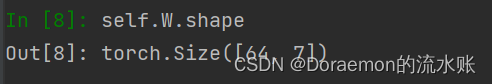
    self.W = nn.Parameter(torch.empty(size=(in_features, out_features)))
    nn.init.xavier_uniform_(self.W.data, gain=1.414)
    self.a = nn.Parameter(torch.empty(size=(2*out_features, 1)))  # concat(V,NeigV)
    nn.init.xavier_uniform_(self.a.data, gain=1.414)

    self.leakyrelu = nn.LeakyReLU(self.alpha)

首先是对公式中的W的定义，in_features, out_features分别是(1433,8)，也就是说W是将1433维的特征转换为8维

接着定义了α向量，作为Whi与Whj向量拼接后的系数，因为是横向拼接所以2*out_features

最后定义了leakyrelu激活函数

步出GraphAttentionLayer，进入class GAT(nn.Module)line8的循环，因为样例中定义了8个head，因此循环了8次定义了8个GraphAttentionLayer

self.attentions = [GraphAttentionLayer(nfeat, nhid, dropout=dropout, alpha=alpha, concat=True) for _ in range(nheads)]

定义第二层GraphAttentionLayer

回到class GAT(nn.Module)的init中line11，对第二层（最后一层）GraphAttentionLayer进行定义

self.out_att = GraphAttentionLayer(nhid * nheads, nclass, dropout=dropout, alpha=alpha, concat=False)

这里的nhid * nheads为8*8，也就是隐层维度与注意力头数相乘，nclass=7是最后要映射到的7个类别上，对于这一层的GraphAttentionLayer内部同上，不再赘述

模型训练

进行初始化

在train.py中有对cuda的定义，如果设置了CUDA使用GPU算的时要转换为Variable，因为variable是一种可以不断变化的变量，符合反向传播而tensor不能反向传播

Variable计算时，会逐步生成计算图，这个图将所有的计算节点都连接起来，最后进行loss反向传播时，一次性将所有Variable里的梯度计算出来，然而tensor没有这个能力

train.py

if args.cuda:
    model.cuda()
    features = features.cuda()
    adj = adj.cuda()
    labels = labels.cuda()
    idx_train = idx_train.cuda()
    idx_val = idx_val.cuda()
    idx_test = idx_test.cuda()

features, adj, labels = Variable(features), Variable(adj), Variable(labels)

跟进train()=>model(features, adj)

train.py

def train(epoch):
    t = time.time()
    model.train()
    optimizer.zero_grad()
    output = model(features, adj)  # GAT模块
    loss_train = F.nll_loss(output[idx_train], labels[idx_train])
    acc_train = accuracy(output[idx_train], labels[idx_train])
    loss_train.backward()
    optimizer.step()

再跟进model(features, adj)中的forward

models.py

def forward(self, x, adj):
    x = F.dropout(x, self.dropout, training=self.training)
    x = torch.cat([att(x, adj) for att in self.attentions], dim=1)  # 将每层attention拼接
    x = F.dropout(x, self.dropout, training=self.training)
    x = F.elu(self.out_att(x, adj))   # 第二层的attention layer
    return F.log_softmax(x, dim=1)

也就是在定义好的模型上先进行前向传播，先是第一层的GraphAttentionLayer，在上面line3的self.attentions中步入

走进第一层

layers.py

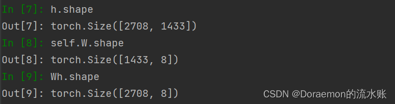
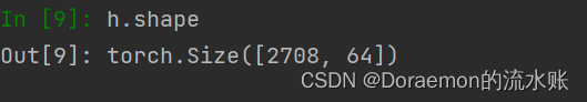
def forward(self, h, adj):
    Wh = torch.mm(h, self.W) # h.shape: (N, in_features), Wh.shape: (N, out_features)
    a_input = self._prepare_attentional_mechanism_input(Wh)  # 每一个节点和所有节点，特征。(Vall, Vall, feature)
    e = self.leakyrelu(torch.matmul(a_input, self.a).squeeze(2))
    # 之前计算的是一个节点和所有节点的attention，其实需要的是连接的节点的attention系数
    zero_vec = -9e15*torch.ones_like(e)
    attention = torch.where(adj > 0, e, zero_vec)    # 将邻接矩阵中小于0的变成负无穷
    attention = F.softmax(attention, dim=1)  # 按行求softmax。 sum(axis=1) === 1
    attention = F.dropout(attention, self.dropout, training=self.training)
    h_prime = torch.matmul(attention, Wh)   # 聚合邻居函数

    if self.concat:
        return F.elu(h_prime)   # elu-激活函数
    else:
        return h_prime

先看上面line2的h和W，不难看出是通过W参数矩阵对1433维度特征的压缩

再看上面line3处的self._prepare_attentional_mechanism_input，跟进后发现比较复杂，还好作者给了解释和说明

layers.py

def _prepare_attentional_mechanism_input(self, Wh):
    N = Wh.size()[0] # number of nodes

    # Below, two matrices are created that contain embeddings in their rows in different orders.
    # (e stands for embedding)
    # These are the rows of the first matrix (Wh_repeated_in_chunks): 
    # e1, e1, ..., e1,            e2, e2, ..., e2,            ..., eN, eN, ..., eN
    # '-------------' -> N times  '-------------' -> N times       '-------------' -> N times
    # 
    # These are the rows of the second matrix (Wh_repeated_alternating): 
    # e1, e2, ..., eN, e1, e2, ..., eN, ..., e1, e2, ..., eN 
    # '----------------------------------------------------' -> N times
    # 
    
    Wh_repeated_in_chunks = Wh.repeat_interleave(N, dim=0)  # 复制
    Wh_repeated_alternating = Wh.repeat(N, 1)
    # Wh_repeated_in_chunks.shape == Wh_repeated_alternating.shape == (N * N, out_features)

    # The all_combination_matrix, created below, will look like this (|| denotes concatenation):
    # e1 || e1
    # e1 || e2
    # e1 || e3
    # ...
    # e1 || eN
    # e2 || e1
    # e2 || e2
    # e2 || e3
    # ...
    # e2 || eN
    # ...
    # eN || e1
    # eN || e2
    # eN || e3
    # ...
    # eN || eN

    all_combinations_matrix = torch.cat([Wh_repeated_in_chunks, Wh_repeated_alternating], dim=1)
    # all_combinations_matrix.shape == (N * N, 2 * out_features)

    return all_combinations_matrix.view(N, N, 2 * self.out_features)

为了计算两个相邻节点的attention，这里面并没有提取相邻节点，而是把全局所有的N个节点都一一配对，出了N*N个对，得到了如下的向量

也就是N*N，2*output_feature，也就是所有节点两两拼接的feature，return到forward(self, h, adj)的line3的a_input

a_input = self._prepare_attentional_mechanism_input(Wh)

但是我们要明确的是，需要求的是相邻节点之间的attention，刚刚上面的只是一个全局的初始化

那么，怎么定义相邻节点的attention呢？

先别着急，接着看，line4其实就是eij

e = self.leakyrelu(torch.matmul(a_input, self.a).squeeze(2))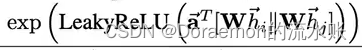

接着初始化了一个负无穷的zero_vec矩阵

zero_vec = -9e15*torch.ones_like(e)

因为之前定义过一个叫adj的邻接矩阵，储存了节点的相连关系，所以对attention是这样定义的

attention = torch.where(adj > 0, e, zero_vec)

通过这一步，将邻接矩阵adj中大于0（有边的）置为刚刚定义的eij，小于0的变成负无穷，可以看一下效果

但是这并不是最终attention的系数，还要通过softmax归一化

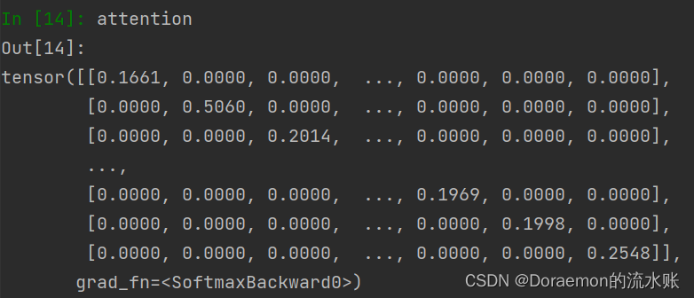
归一化之后的attention，每一个节点对行求和之后系数是1，也就很好的说明了相邻节点对于目标节点的权重系数之和为1

求完了attention之后，来求

也就是

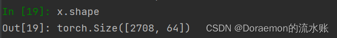
h_prime = torch.matmul(attention, Wh) # 聚合邻居函数

得到了表示2708个节点隐层的矩阵

又因为定义了8个attention的head，这里循环了8次使用

x = torch.cat([att(x, adj) for att in self.attentions], dim=1) # 将8层attention拼接

也就是

好，Dropout之后，到此，第一层就结束了

走进第二层

再回到model(features, adj)中的forward的line5

x = F.elu(self.out_att(x, adj))

也就是第二层的GraphAttentionLayer，h是刚刚拼好的x

因为最后是7分类，所以这里W的维度有所不同

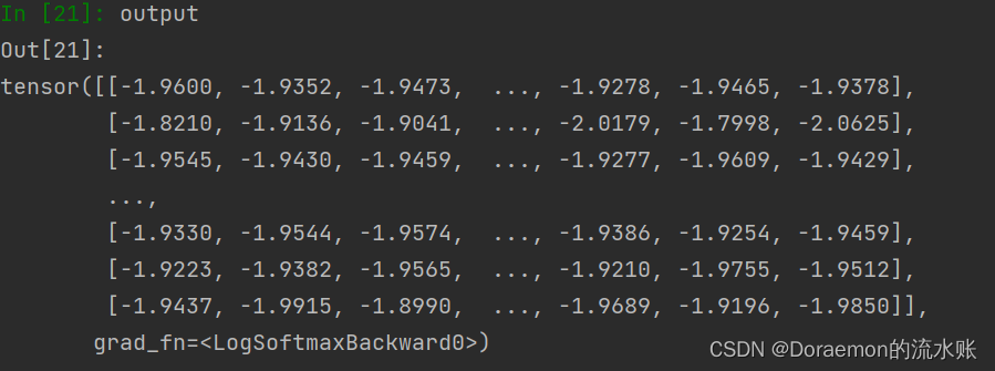
其他部分没有什么变化，第二层最终输出的就是，接上一个softmax输出为output

再贴一遍train

train.py

def train(epoch):
    t = time.time()
    model.train()
    optimizer.zero_grad()
    output = model(features, adj)  # GAT模块
    loss_train = F.nll_loss(output[idx_train], labels[idx_train])
    acc_train = accuracy(output[idx_train], labels[idx_train])
    loss_train.backward()
    optimizer.step()

上面的line6的nll_loss怎么理解？其实就是nn.CrossEntropyLoss