Attention is all you need文章翻译

近期读完了经典文章《Attention Is All You Need》，发表在第31届神经信息处理系统会议上（31st Conference on Neural Information Processing Systems, NIPS 2017, Long Beach, CA, USA）有挺多地方还是一知半解的，这里再次翻译一遍，加深理解也留下一些材料

文章有8个联合作者，主要是来自谷歌团队的大佬们。在论文首页的注释中，注明了所有作者对研究有相同的贡献，不同人有不同的分工。

训练以及结果部分不翻译

整理不易，转载请注明出处
如有疏漏请务必指出

Abstract 摘要

主导性的序列转导模型都是基于包括一个编码器和一个解码器的复杂的循环（recurrent）或者卷积神经网络。性能最好的模型也会使用attention机制连接编码器解码器。我们提出了一种新的简单地网络结构，Transformer，结构仅仅基于注意力机制，无需循环以及卷积结构。在两个机器翻译任务上实验显示，这些模型在翻译质量上更加优越，同时模型并行化程度更高，需要的训练时间更短。我们的模型在WMT 2014英语翻译德语的翻译任务上达到了28.4 BLEU的成绩，从包括ensembels的最好的结果上提升了超过2个BLEU。在WMT 2014英语德语翻译任务上，我们的模型在8块GPU上训练了3.5天后建立了新的单模型SOTA 41.0 BLEU的分数， a small fraction of the training costs of the best models from the literature。

1.Introduction 介绍

循环神经网络，长短记忆（long short-term）以及特别的门控循环（gated recurrent）神经网络，已经牢固地在类似于语言建模（language modeling）以及机器翻译（machine translation）的序列建模（sequence modeling）以及转导问题（transduction problems）中，建立了SOTA的方法。从那之后，大量的研究继续推动了循环语言模型以及编码器解码器架构的边界。

循环模型基本上将沿着输入输出序列符号位置的计算作为考虑因素，将位置调整为计算时间中的步骤，他们生成了一个隐藏状态$h_i$的序列，作为前一时刻隐藏状态$h_{t-1}$以及输入位置$t$的方程。这种内在的序列特性妨碍了对训练样本的平行计算，这在序列长度更长的时候会变得更加严重，因为memory constraints限制了对所有样本的batching。近期的工作通过factorization（因子分解）技巧以及条件计算（conditional computation）显著地提升了计算效率，对于后者还提升了模型性能。然而序列计算的根本constraint依然存在。

注意力机制（Attention mechanisms）已经成为了多种任务的序列建模以及转导模型的一部分（integral part），允许了在对dependencies建模时不需要估计他们在输入输出中的距离。在了小部分的情况下，这样的注意力机制还与循环网络一同使用。

在这片文章里，我们提出了Transformer，一个避免循环的的结构，完全依靠一个注意力机制在输入输出之间建立全局的dependencies。Transformer显著地提升了计算平行度，在8块GPU上训练了12小时那么少的时间，就达到了新的SOTA翻译质量。

2.Background 背景

减少顺序计算的目标也构成了Extended Neural GPU [20]、ByteNet [15] 和 ConvS2S [8] 的基础，所有这些都使用卷积神经网络作为基本构建块，并行计算所有输入和输出位置。在这些模型中，关联来自两个任意输入或输出位置的信号所需的操作数量随着位置之间的距离而增加，对于 ConvS2S 是线性增长，对于 ByteNet 是对数

（logarithmically）增长。这使得学习远距离位置之间的依赖关系变得更加困难 [11]。在 Transformer 中，操作数量被减少到恒定数量的操作，尽管代价是由于平均注意力加权的位置而导致有效分辨率降低，我们用 3.2 节中描述的Multi-Head Attention（多头注意力）来抵消这种影响。

Self-attention（自注意），有时也称为intra-attention（内部注意），是一种将单个序列的不同位置关联起来以计算序列表示的注意机制。自注意力已成功用于各种任务，包括阅读理解、抽象摘要（ abstractive summarization）、文本蕴涵（textual entailment）和学习与任务无关（task-independence）的句子表示 [4, 22, 23, 19]。

端到端记忆网络基于循环注意机制而不是序列对齐循环，并且已被证明在简单语言问答和语言建模任务中表现良好[28]。

然而，据我们所知，Transformer 是第一个完全依赖自注意力来计算其输入和输出表示而不使用序列对齐 RNN 或卷积的转导模型。在接下来的部分中，我们将描述 Transformer，解释（motivate）自我注意并讨论它相对于 [14, 15] 和 [8] 等模型的优势。

3.Model Architecture模型架构

大多数具有竞争力的神经序列转导模型都具有编码器-解码器结构 [5, 2, 29]。 在这里，编码器将输入的符号（symbol）$(x_1,...,x_n)$映射到连续的表示序列$z=(z_1,...,z_n)$。 给定$z$，解码器然后生成一个符号（symbol）的输出序列$(y_1,...,y_m)$，一次一个元素。 在每一步，模型都是自回归的（auto-regressive）[9]，在生成下一个时，将先前生成的符号（symbols）作为附加输入使用。

Transformer 遵循这种整体架构，为编码器和解码器使用堆叠的自注意力和逐点的全连接层，分别如图 1 的左半部分和右半部分所示。

图1：Transformer模型架构

3.1 Encoder and Decoder Stacks 编解码器堆

编码器：编码器包括6个独立的层（layers）的堆栈。每一层都有两个子层。第一个是一个多头的自注意力机制，第二个是一个简单地逐位置的全连接前馈网络（position-wise fully connected feed-forward network）。我们在两个子层的每一个周围都使用了一个残差连接 [10]，然后是层归一化 [1]。 即每个子层的输出是$LayerNorm(x+Sublayer(x))$，其中$Sublayer(x)$是通过子层自己实现的函数。 为了使这些残差连接更易实现，模型中的所有子层以及嵌入层产生维度$d_{model}=512$的输出。

解码器：解码器也由 N = 6 个相同层（layers）的堆栈组成。 除了每个编码器层中的两个子层之外，解码器还插入了第三个子层，该子层对编码器堆栈的输出执行多头注意力机制。 与编码器类似，我们在每个子层周围部署残差连接，然后进行层归一化。 我们还修改了解码器堆栈中的自注意力子层， to prevent positions from attending to subsequent positions（以防止位置关注后续位置）。 这种掩码与输出embedding偏移一个位置的事实相结合，确保位置$i$的预测只能依赖于小于$i$位置的已知输出。

3.2 Attention 注意力

注意力函数可以描述为将一个query和一组key-value对映射到一个output，其中query、keys、values和output都是向量。 output计算为values的加权总和，其中分配给每个value的权重由query与相应key的兼容性函数（compatibility function）计算。

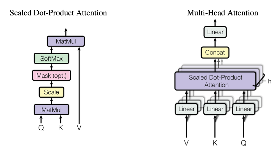
3.2.1 Scaled Dot-Product Attention

我们将我们独特的Attention称为“Scaled Dot-Product Attention”（图 2）。 输入由$d_k$维度的queries和keys以及$d_v$维度的values组成。 我们使用所有keys对querys计算点积，将每个点积结果除以$\sqrt{d_k}$，然后应用 softmax 函数来获取values的权重。

在实践中，我们同时计算一组querys的注意力函数，将它们打包成一个矩阵$Q$。keys和values也一起打包成矩阵$K$和$V$。 我们这样计算输出矩阵：
$$Attention(Q,K,V)=softmax(\frac{Q{K}^T}{\sqrt{d_k}})V\text{\hspace{1em}(1)}$$
两个最常用的注意力函数是additive注意力[2]和点积（乘法）注意力。 除了缩放因子$\frac{1}{sqrt{d}_k}$之外，点积注意力与我们的算法是一致的。 additive注意力使用带有一个隐藏层的前馈网络计算兼容性函数（compatibility function）。 虽然两者在理论复杂度上相似，但点积注意力在实践中速度更快，空间效率更高，因为它可以使用高度优化的矩阵乘法代码来实现

虽然对于较小的$d_k$值，这两种机制的相似表现性能，但对于更大的$d_k$，addictive注意力优于没有缩放的点积注意力[3]。我们怀疑对于较大的$d_k$值，点积的量级增长很大，将 softmax 函数推入梯度极小的区域⁴。为了抵消中和(counteract)这种影响，我们将点积缩放$\frac{1}{sqrt{d}_k}$

图2：(左)Scaled Dot-Product Attention. (右)包含几个并行计算注意力层的Multi-Head Attention

⁴ 为了说明点积变大的原因，假设$q$和$k$的分量是独立随机的 均值为0且方差为1的变量。那么它们的点积$q\cdot k={\sum }_{t=1}^{d_k}{q}_i{k}_i$，均值为0，方差为$d_k$。

3.2.2 Multi-Head Attention 多头注意力

与使用$d_{model}$维度的keys、values和queries执行单个注意力函数不同，我们发现这样是有益的：使用不同的学习到的线性投影，将queries、keys和values分别线性投影$h$次到$d_k$、$d_k$和$d_v$维。对每一个投影过后的queries、keys和values上，我们接着并行地执行注意力功能，获得$d_v$维输出values。 这些values被连接并再次投影，从而产生最终values，如图 2 所示。
多头注意力允许模型共同(jointly)关注来自不同位置的不同表示子空间的信息。 使用单个注意力头，其平均作用会抑制这种情况。
$$\begin{array}{r}MultiHead(Q,K,V)=Concat(hea{d}_1,...,hea{d}_h)W^O\\ \\ wherehea{d}_i=Attention(Q{W}_i^Q,Q{W}_i^K,Q{W}_i^V）\end{array}$$

其中投影是参数矩阵$W_i^Q\in {\mathbb{R}}^{d\_model\times d_k}$，$W_i^K\in {\mathbb{R}}^{d\_model\times d_k}$，$W_i^V\in {\mathbb{R}}^{d\_model\times d_v}$和$W_i^O\in {\mathbb{R}}^{hd\_v\times d_{model}}$。

在这项工作中，我们使用了$h=8$个平行的注意力层或头。 对于其中的每一个，我们使用$d_k=d_v=d_{model}/h=64$。由于每个头维度的减少，总计算成本类似于具有全维度的单头注意力。

3.2.3 Applications of Attention in our Model 我们模型中注意力的应用

Transformer 以三种不同的方式使用多头注意力：

• 在“编码器-解码器注意力”层中，queries来自前一个解码器层，记忆keys和values来自编码器的输出。 这允许解码器中的每个位置都参与输入序列中的所有位置。 这模仿了序列到序列模型中典型的编码器-解码器注意机制，例如 [31, 2, 8]。
• 编码器包含自注意层。 在自注意力层中，所有的keys、values和queries都来自同一个地方，在本文中，是编码器上一层的输出。 编码器中的每个位置都可以参与(attend to)编码器前一层中的所有位置。
• 类似地，解码器中的自注意力层允许解码器中的每个位置关注解码器中直到当前并包括当前位置的所有位置。 我们需要防止解码器中被留下的(left)信息流以保留自回归特性。 我们通过屏蔽（设置为$-\infty$）softmax 输入中所有与非法连接相对应的values，来在Scaled Dot-Production内部实现这一点。 见图 2。

3.3 Position-wise Feed-Forward Nerworks 逐位置的前馈网络

除了子注意力层之外，我们的编码器和解码器中的每一层都包含一个全连接前馈网络，该网络在每个位置结构相同且独立部署。这由两个线性变换组成，中间有一个 ReLU激活。
$$FPN(x)=max(0,x{W}_1+b_1)W_2+b_2\text{\hspace{1em}(2)}$$
虽然不同位置的线性变换是相同的，但它们在不同层中使用不同的参数。 另一种描述方式是两个核大小为1的卷积层。输入和输出的维度为$d_{model}=512$，内层的维度为$d_{ff}=2048$。

3.4 Embedding and Softmax 嵌入层以及softmax

与其他序列转导模型类似，我们使用学习的嵌入(learned embeddings)将输入tokens和输出tokens转换为维度$d\_model$的向量。我们还使用正常学习到的线性变换和 softmax 函数，将解码器输出进行转换，预测next-token概率。 在我们的模型中，我们在两个嵌入层和 pre-softmax 线性变换之间共享相同的权重矩阵，类似于 [24]。 在嵌入层中，我们将这些权重乘以$\sqrt{d_{model}}$。

3.5 Positional Encoding 位置编码

由于我们的模型不包含递归和卷积，为了让模型利用序列的顺序信息，我们必须注入一些关于tokens在序列中的相对或绝对位置的信息。为此，我们将“位置编码(positional encodings)”添加到编码器和解码器堆栈底部的输入嵌入中。位置编码与嵌入具有相同的维度$d_{model}$，因此可以将两者相加。 位置编码有多种选择，学习的和固定的 [8]。

这篇文章中，我们使用不同频率的sine以及cosine函数
$$\begin{array}{r}P{E}_{(pos,2i)}=sin(\frac{pos}{10000^{\frac{2i}{d_{model}}}})\\ \\ P{E}_{(pos,2i+1)}=cos(\frac{pos}{10000^{\frac{2i}{d_{model}}}})\end{array}$$

译者注：这里可以看到，不同维度的频率是不一样的

其中$pos$是位置，$i$是维度。 也就是说，位置编码的每个维度对应一个正弦曲线。 波长形成从$2\pi$到$10000\cdot 2\pi$的几何级数。 我们选择这个函数是因为我们假设它可以让模型在伴随相对位置信息的情况下能够轻松学习（这句不太理解：because we hypothesized it would allow the model to easily learn to attend by relative positions），因为对于任何固定的偏移量$k$，$P{E}_{pos+k}$可以表示为$P{E}_{pos}$的线性函数。

我们还尝试使用学习的位置嵌入 [8]，发现两个版本产生了几乎相同的结果（见表 3 行 (E)）。 我们选择了正弦版本，因为它可能允许模型外推(extrapolate)到比训练期间遇到的序列长度更长的序列长度。

4. Why Self-Attention 为什么使用自注意力

在本节中，我们将自注意力层的各个方面与递归及卷积层做对比，这些递归及卷积层通常用于将一个可变长度的符号表示序列$(x_1,...,x_n)$映射到另一个等长序列$(z_1,......,z_n)$，其中$x_i,z_i\in {\mathbb{R}}_d$，例如典型序列转导编码器或解码器中的隐藏层。我们考虑三个需求激励我们使用自注意。

一个是每层的总计算复杂度。另一个是可以并行化的计算量，通过所需的最小顺序操作数来衡量。

第三个是网络中远程依赖之间的路径长度。学习远程依赖是许多序列转导任务中的关键挑战。影响学习这种依赖性能力的一个关键因素是前向和后向信号必须在网络中穿越的路径长度。输入和输出序列中任意位置组合之间的这些路径越短，学习远程依赖关系就越容易[11]。因此，我们还比较了由不同层类型组成的网络中任意两个输入和输出位置之间的最大路径长度。

表 1：不同层类型的最大路径长度、每层复杂度和最小顺序操作数。$n$是序列长度，$d$是表示维度，$k$是卷积核大小，$r$是受限自注意力中的邻域大小。

Layer Type 层类型	Complexity per Layer 每层的复杂度	Sequential Operations 顺序操作数	Maximum Path Length 最大路径长度
Self-Attention 自注意力	$O(n^2\cdot d)$	$O(1)$	$O(1)$
Recurrent 循环结构	$O(n\cdot d^2)$	$O(n)$	$O(n)$
Convolutional 卷积	$O(k\cdot n\cdot d^2)$	$O(1)$	$O({\log }_k(n))$
Self-Attention(restricted) 自注意力(被限制)	$O(r\cdot n\cdot d)$	$O(1)$	$O(n/r)$

如表 1 所示，自注意力层将所有位置连接到具有恒定数量的顺序执行操作，而循环层需要$O(n)$顺序操作。在计算复杂度方面，当序列长度$n$小于表示维数（这里指的是输入序列经过嵌入映射后的表示）$d$时，自注意力层比循环层更快，这是机器翻译中最先进模型使用的句子表示的最常见情况，例如word-piece [31] 和byte-pair [25] 表示。为了提高涉及非常长序列的任务的计算性能，可以将自注意力限制为仅考虑输入序列中以相应输出位置为中心的大小为$r$的邻域。这会将最大路径长度增加到$O(n/r)$。我们计划在未来的工作中进一步研究这种方法。

内核宽度$k<n$的单个卷积层不会连接所有输入和输出位置对。这样做在增加网络中任意两个位置之间最长路径的长度时，需要在连续内核的情况下堆叠$O(n/k)$卷积层，或者在扩张卷积的情况下需要$O(lo{g}_k(n))$[15]。卷积层通常比循环层成本高出$k$倍。然而，可分离卷积 [6] 将复杂度显着降低到$O(k\cdot n\cdot d+n\cdot d^2)$。然而，即使$k=n$，可分离卷积的复杂性也等于自我注意层和逐点前馈层的组合，我们在我们的模型中采用的方法。

作为附带好处，self-attention 可以产生更多可解释的模型。我们从我们的模型中检查注意力分布，并在附录中展示和讨论示例。单个注意力头不仅清楚地学习执行不同的任务，而且许多人似乎表现出与句子的句法和语义结构相关的行为。

5. Train

This section describes the training regime for our models.

5.1 Training Data and Batching

We trained on the standard WMT 2014 English-German dataset consisting of about 4.5 million sentence pairs. Sentences were encoded using byte-pair encoding [3], which has a shared source- target vocabulary of about 37000 tokens. For English-French, we used the significantly larger WMT 2014 English-French dataset consisting of 36M sentences and split tokens into a 32000 word-piece vocabulary [31]. Sentence pairs were batched together by approximate sequence length. Each training batch contained a set of sentence pairs containing approximately 25000 source tokens and 25000 target tokens.

5.2 Hardware and Schedule

We trained our models on one machine with 8 NVIDIA P100 GPUs. For our base models using the hyperparameters described throughout the paper, each training step took about 0.4 seconds. We trained the base models for a total of 100,000 steps or 12 hours. For our big models,(described on the bottom line of table 3), step time was 1.0 seconds. The big models were trained for 300,000 steps (3.5 days).

5.3 Optimizer

We used the Adam optimizer [17] with${\beta }_1=0.9,{\beta }_2=0.98$and$ϵ=10^{-9}$. We varied the learning rate over the course of training, according to the formula:
$$lrate=d_{model}^{-0.5}\cdot min(step\_nu{m}^{0.5},step\_num\cdot warmu{p}_{s}tep{s}^{-1.5})\text{\hspace{1em}(3)}$$
This corresponds to increasing the learning rate linearly for the first warmup_steps training steps, and decreasing it thereafter proportionally to the inverse square root of the step number. We used$warmu{p}_{s}teps=4000$.

5.4 Regularization

We employ three types of regularization during training:

Residual Dropout We apply dropout [27] to the output of each sub-layer, before it is added to the sub-layer input and normalized. In addition, we apply dropout to the sums of the embeddings and the positional encodings in both the encoder and decoder stacks. For the base model, we use a rate of$P_{drop}=0.1$.

Table 2: The Transformer achieves better BLEU scores than previous state-of-the-art models on the English-to-German and English-to-French newstest2014 tests at a fraction of the training cost.

Label Smoothing During training, we employed label smoothing of value εls = 0.1 [30]. This hurts perplexity, as the model learns to be more unsure, but improves accuracy and BLEU score.

6. Results

6.1 Machine Translation

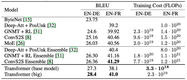
On the WMT 2014 English-to-German translation task, the big transformer model (Transformer (big) in Table 2) outperforms the best previously reported models (including ensembles) by more than 2.0 BLEU, establishing a new state-of-the-art BLEU score of 28.4. The configuration of this model is listed in the bottom line of Table 3. Training took 3.5 days on 8 P100 GPUs. Even our base model surpasses all previously published models and ensembles, at a fraction of the training cost of any of the competitive models.

On the WMT 2014 English-to-French translation task, our big model achieves a BLEU score of$41.0$, outperforming all of the previously published single models, at less than 1/4 the training cost of the previous state-of-the-art model. The Transformer (big) model trained for English-to-French used dropout rate$P_{drop}=0.1$, instead of$0.3$.

For the base models, we used a single model obtained by averaging the last 5 checkpoints, which were written at 10-minute intervals. For the big models, we averaged the last 20 checkpoints. We used beam search with a beam size of 4 and length penalty$\alpha =0.6$[31]. These hyperparameters were chosen after experimentation on the development set. We set the maximum output length during inference to input length$+50$, but terminate early when possible [31].

Table 2 summarizes our results and compares our translation quality and training costs to other model architectures from the literature. We estimate the number of floating point operations used to train a model by multiplying the training time, the number of GPUs used, and an estimate of the sustained single-precision floating-point capacity of each GPU⁵.

⁵We used values of 2.8, 3.7, 6.0 and 9.5 TFLOPS for K80, K40, M40 and P100, respectively.

6.2 Model Variations

To evaluate the importance of different components of the Transformer, we varied our base model in different ways, measuring the change in performance on English-to-German translation on the development set, newstest2013. We used beam search as described in the previous section, but no checkpoint averaging. We present these results in Table 3.

In Table 3 rows (A), we vary the number of attention heads and the attention key and value dimensions, keeping the amount of computation constant, as described in Section 3.2.2. While single-head attention is 0.9 BLEU worse than the best setting, quality also drops off with too many heads.

Table 3: Variations on the Transformer architecture. Unlisted values are identical to those of the base model. All metrics are on the English-to-German translation development set, newstest2013. Listed perplexities are per-wordpiece, according to our byte-pair encoding, and should not be compared to per-word perplexities.

In Table 3 rows (B), we observe that reducing the attention key size dk hurts model quality. This suggests that determining compatibility is not easy and that a more sophisticated compatibility function than dot product may be beneficial. We further observe in rows (C) and (D) that, as expected, bigger models are better, and dropout is very helpful in avoiding over-fitting. In row (E) we replace our sinusoidal positional encoding with learned positional embeddings [8], and observe nearly identical results to the base model.

7. Conclusion 结论

在这项工作中，我们提出了 Transformer，这是第一个完全基于注意力的序列转换模型，用多头自注意力取代了编码器-解码器架构中最常用的循环层。

对于翻译任务，Transformer 的训练速度明显快于基于循环或卷积层的架构。 在 WMT 2014 English-to-German 和 WMT 2014 English-to-French 翻译任务中，我们达到了最先进的水平。 在前一个任务中，我们最好的模型甚至优于所有先前报告的集成。

我们对基于注意力模型的未来感到兴奋，并计划将它们应用于其他任务。 我们计划将 Transformer 扩展到涉及文本以外的输入和输出模式的问题，并研究局部、受限的注意力机制以有效处理大型输入和输出，如图像、音频和视频。 减少生成过程的连续性是我们的另一个研究目标。

我们用来训练和评估的模型代码在这里提供https://github.com/tensorflow/tensor2tensor.

致谢 我们感谢 Nal Kalchbrenner 和 Stephan Gouws 富有成果的评论、更正和启发。

References 参考文献

[1] Jimmy Lei Ba, Jamie Ryan Kiros, and Geoffrey E Hinton. Layer normalization. arXiv preprint arXiv:1607.06450, 2016.

[2] Dzmitry Bahdanau, Kyunghyun Cho, and Yoshua Bengio. Neural machine translation by jointly learning to align and translate. CoRR, abs/1409.0473, 2014.

[3] Denny Britz, Anna Goldie, Minh-Thang Luong, and Quoc V. Le. Massive exploration of neural machine translation architectures. CoRR, abs/1703.03906, 2017.

[4] Jianpeng Cheng, Li Dong, and Mirella Lapata. Long short-term memory-networks for machine reading. arXiv preprint arXiv:1601.06733, 2016.

[5] Kyunghyun Cho, Bart van Merrienboer, Caglar Gulcehre, Fethi Bougares, Holger Schwenk, and Yoshua Bengio. Learning phrase representations using rnn encoder-decoder for statistical machine translation. CoRR, abs/1406.1078, 2014.

[6] Francois Chollet. Xception: Deep learning with depthwise separable convolutions. arXiv preprint arXiv:1610.02357, 2016.

[7] Junyoung Chung, Çaglar Gülçehre, Kyunghyun Cho, and Yoshua Bengio. Empirical evaluation of gated recurrent neural networks on sequence modeling. CoRR, abs/1412.3555, 2014.

[8] Jonas Gehring, Michael Auli, David Grangier, Denis Yarats, and Yann N. Dauphin. Convolu- tional sequence to sequence learning. arXiv preprint arXiv:1705.03122v2, 2017.

[9] Alex Graves. Generating sequences with recurrent neural networks. arXiv preprint arXiv:1308.0850, 2013.

[10] Kaiming He, Xiangyu Zhang, Shaoqing Ren, and Jian Sun. Deep residual learning for im- age recognition. In Proceedings of the IEEE Conference on Computer Vision and Pattern Recognition, pages 770–778, 2016.

[11] Sepp Hochreiter, Yoshua Bengio, Paolo Frasconi, and Jürgen Schmidhuber. Gradient flow in recurrent nets: the difficulty of learning long-term dependencies, 2001.

[12] Sepp Hochreiter and Jürgen Schmidhuber. Long short-term memory. Neural computation, 9(8):1735–1780, 1997.

[13] Rafal Jozefowicz, Oriol Vinyals, Mike Schuster, Noam Shazeer, and Yonghui Wu. Exploring the limits of language modeling. arXiv preprint arXiv:1602.02410, 2016.

[14] Łukasz Kaiser and Ilya Sutskever. Neural GPUs learn algorithms. In International Conference on Learning Representations (ICLR), 2016.

[15] Nal Kalchbrenner, Lasse Espeholt, Karen Simonyan, Aaron van den Oord, Alex Graves, and Ko- ray Kavukcuoglu. Neural machine translation in linear time. arXiv preprint arXiv:1610.10099v2, 2017.

[16] Yoon Kim, Carl Denton, Luong Hoang, and Alexander M. Rush. Structured attention networks. In International Conference on Learning Representations, 2017.

[17] Diederik Kingma and Jimmy Ba. Adam: A method for stochastic optimization. In ICLR, 2015.

[18] Oleksii Kuchaiev and Boris Ginsburg. Factorization tricks for LSTM networks. arXiv preprint

arXiv:1703.10722, 2017.

[19] Zhouhan Lin, Minwei Feng, Cicero Nogueira dos Santos, Mo Yu, Bing Xiang, Bowen Zhou, and Yoshua Bengio. A structured self-attentive sentence embedding. arXiv preprint arXiv:1703.03130, 2017.

[20] Samy Bengio Łukasz Kaiser. Can active memory replace attention? In Advances in Neural Information Processing Systems, (NIPS), 2016.

[21] Minh-Thang Luong, Hieu Pham, and Christopher D Manning. Effective approaches to attention- based neural machine translation. arXiv preprint arXiv:1508.04025, 2015.

[22] Ankur Parikh, Oscar Täckström, Dipanjan Das, and Jakob Uszkoreit. A decomposable attention model. In Empirical Methods in Natural Language Processing, 2016.

[23] Romain Paulus, Caiming Xiong, and Richard Socher. A deep reinforced model for abstractive summarization. arXiv preprint arXiv:1705.04304, 2017.

[24] Ofir Press and Lior Wolf. Using the output embedding to improve language models. arXiv preprint arXiv:1608.05859, 2016.

[25] Rico Sennrich, Barry Haddow, and Alexandra Birch. Neural machine translation of rare words with subword units. arXiv preprint arXiv:1508.07909, 2015.

[26] Noam Shazeer, Azalia Mirhoseini, Krzysztof Maziarz, Andy Davis, Quoc Le, Geoffrey Hinton, and Jeff Dean. Outrageously large neural networks: The sparsely-gated mixture-of-experts layer. arXiv preprint arXiv:1701.06538, 2017.

[27] Nitish Srivastava, Geoffrey E Hinton, Alex Krizhevsky, Ilya Sutskever, and Ruslan Salakhutdi- nov. Dropout: a simple way to prevent neural networks from overfitting. Journal of Machine Learning Research, 15(1):1929–1958, 2014.

[28] Sainbayar Sukhbaatar, arthur szlam, Jason Weston, and Rob Fergus. End-to-end memory networks. In C. Cortes, N. D. Lawrence, D. D. Lee, M. Sugiyama, and R. Garnett, editors, Advances in Neural Information Processing Systems 28, pages 2440–2448. Curran Associates, Inc., 2015.

[29] Ilya Sutskever, Oriol Vinyals, and Quoc VV Le. Sequence to sequence learning with neural networks. In Advances in Neural Information Processing Systems, pages 3104–3112, 2014.

[30] Christian Szegedy, Vincent Vanhoucke, Sergey Ioffe, Jonathon Shlens, and Zbigniew Wojna. Rethinking the inception architecture for computer vision. CoRR, abs/1512.00567, 2015.

[31] Yonghui Wu, Mike Schuster, Zhifeng Chen, Quoc V Le, Mohammad Norouzi, Wolfgang Macherey, Maxim Krikun, Yuan Cao, Qin Gao, Klaus Macherey, et al. Google’s neural machine translation system: Bridging the gap between human and machine translation. arXiv preprint arXiv:1609.08144, 2016.

[32] Jie Zhou, Ying Cao, Xuguang Wang, Peng Li, and Wei Xu. Deep recurrent models with fast-forward connections for neural machine translation. CoRR, abs/1606.04199, 2016.

附录需要单独搜索，这里不附上了