opencv的使用技巧（3）

模板匹配
matchTemplate 函数：在模板和输入图像之间寻找匹配,获得匹配结果图像
minMaxLoc 函数：在给定的矩阵中寻找最大和最小值，并给出它们的位置
1. 差值平方和匹配 CV_TM_SQDIFF
2. 标准化差值平方和匹配 CV_TM_SQDIFF_NORMED
3. 相关匹配 CV_TM_CCORR
4. 标准相关匹配 CV_TM_CCORR_NORMED
5. 相关匹配 CV_TM_CCOEFF
6. 标准相关匹配 CV_TM_CCOEFF_NORMED

template = cv2.imread("part.png")  # 读取模板的图
# 模板匹配
h, w = template.shape[:2]  # 获取模板的宽高


#一种方法
result = cv2.matchTemplate(img, template, 0)  # 匹配模板
min_val, max_val, min_loc, max_loc = cv2.minMaxLoc(result)  # 获得匹配图最大阻值最小值的位置
left_top = min_loc  # 左上角的位置就是最小值
right_bottom = (left_top[0] + w, left_top[1] + h)  # 获取右下角的点，0是第一个位置的元素，1是第二个
cv2.rectangle(img, left_top, right_bottom, (0, 255, 0), 2)  # 颜色,粗细,#绘制矩形框


cv2.imshow("src", img)
cv2.imshow("template", template)
cv2.waitKey(0)
cv2.destroyAllWindows()




methods = ["cv2.TM_CCOEFF","cv2.TM_CCOEFF_NORMED","cv2.TM_CCORR","cv2.TM_CCORR_NORMED","cv2.TM_SQDIFF","cv2.TM_SQDIFF_NORMED"]
for meth in methods:
    img2 = img.copy()


    # 匹配方法的真值
    method = eval(meth)
    res = cv2.matchTemplate(img, template, method)
    min_val, max_val, min_loc, max_loc = cv2.minMaxLoc(res)


    # 如果是平方差匹配TM_SQDIFF或归一化平方差匹配TM_SQDIFF_NORMED，取最小值
    if method in [cv2.TM_SQDIFF, cv2.TM_SQDIFF_NORMED]:
        top_left = min_loc
    else:
        top_left = max_loc
    bottom_right = (top_left[0] + w, top_left[1] + h)




    # 画矩形
    cv2.rectangle(img2, top_left, bottom_right, (255,0,0), 4)


    plt.subplot(121), plt.imshow(res, cmap='gray')
    plt.xticks([]), plt.yticks([])  # 隐藏坐标轴
    plt.subplot(122), plt.imshow(img2, cmap='gray')
    plt.xticks([]), plt.yticks([])
    plt.suptitle(meth)
    plt.show()

多对象匹配

img_rgb = cv2.imread('more.png')
img_gray = cv2.cvtColor(img_rgb, cv2.COLOR_BGR2GRAY)
template = cv2.imread('less.png', 0)
h, w = template.shape[:2]


res = cv2.matchTemplate(img_gray, template, cv2.TM_CCOEFF_NORMED)
threshold = 0.4
# 取匹配程度大于%80的坐标
loc = np.where(res >= threshold)
#np.where返回的坐标值(x,y)是(h,w)，注意h,w的顺序
for pt in zip(*loc[::-1]):
    bottom_right = (pt[0] + w, pt[1] + h)
    cv2.rectangle(img_rgb, pt, bottom_right, (0, 0, 255), 2)


cv2.imshow('img_rgb', img_rgb)
cv2.waitKey(0)

直方图
calcHist-计算图像直方图
函数原型：calcHist(images,channels,mask,histSize,ranges,hist=None,accumulate=None)
images：图像矩阵，例如：[image]
channels：通道数，例如：0
mask：掩膜，一般为：None
histSize：直方图大小，一般等于灰度级数
ranges：横轴范围

#直方图
img = cv2.imread("cat.jpg",0) #0表示灰度图
hist = cv2.calcHist([img],[0],None,[256],[0,256])
print(hist.shape)  #256个可能取值 0~255
plt.hist(img.ravel(),256);
plt.show()


#彩色图
img = cv2.imread("cat.jpg")
color = ("b","g","r")
for i,col in enumerate(color):
    histr = cv2.calcHist([img],[i],None,[256],[0,256])
    plt.plot(histr,color = col)
    plt.xlim([0,256])


plt.show()

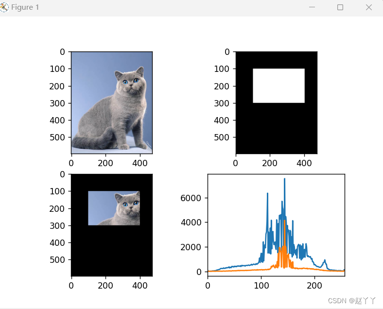
掩膜

mask = np.zeros(img.shape[:2],np.uint8) #指定图像大小，无符号整型
mask[100:300,100:400] = 255 #选择区域 保存白色
masked_img = cv2.bitwise_and(img,img,mask=mask) #与操作
#掩膜的直方图和原图的直方图
hist_full = cv2.calcHist([img],[0],None,[256],[0,256])
hist_mask = cv2.calcHist([img],[0],mask,[256],[0,256])
plt.subplot(221),plt.imshow(img)
plt.subplot(222),plt.imshow(mask,"gray")
plt.subplot(223),plt.imshow(masked_img,"gray")
plt.subplot(224),plt.plot(hist_full),plt.plot(hist_mask)
plt.xlim([0,256])
plt.show()

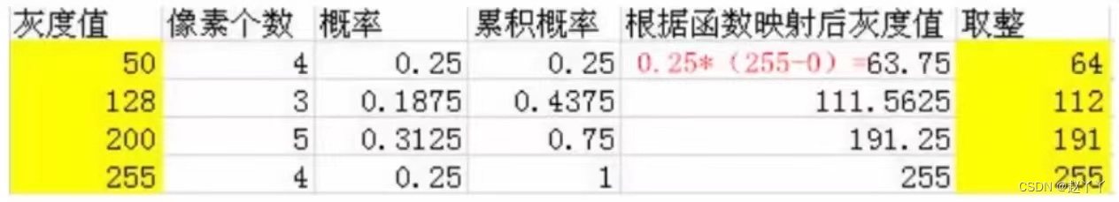
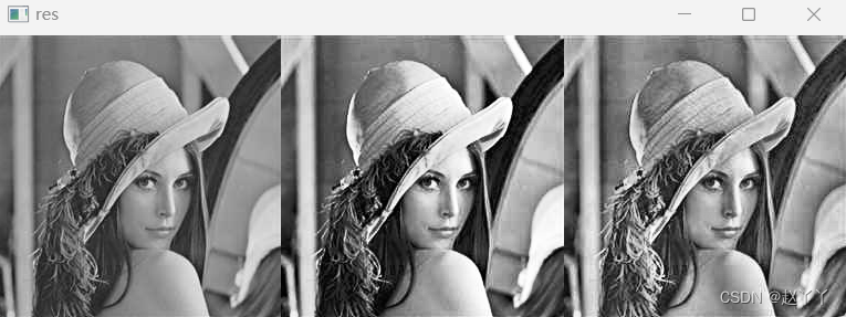
直方图均衡化

img = cv2.imread("lean.jpg",0)
plt.hist(img.ravel(),256)
#均衡化
equ = cv2.equalizeHist(img)
# plt.hist(equ.ravel(),256)
# plt.show()
#
# res = np.hstack((img,equ))
# cv2.imshow("res",res)
# cv2.waitKey(0)
# cv2.destroyAllWindows()


#自适应直方图均衡化 创建一些小格子，通过小格子自己做自己的
clahe = cv2.createCLAHE(clipLimit=2.0,tileGridSize=(8,8))
res_clahe = clahe.apply(img)
res = np.hstack((img,equ,res_clahe))
cv2.imshow("res",res)
cv2.waitKey(0)
cv2.destroyAllWindows()

傅里叶变换的作用
高频：变化剧烈的灰度分量，例如：边界
低频：变化缓慢的灰度分量，例如：一片大海
滤波：
低通滤波器：只保留低频，会使图像模糊
高通滤波器：只保留高频，会使得图像细节增强
主要就是cv2.dft()和cv2.idft()，输入图像需要先转换成np.float32格式
得到的结果中频率为0的部分会在左上角，通常要转换到中心位置，可以通过shift变换来实现
cv2.dft()返回的结果是双通道的（实部，虚部），通常还需要转换成图像格式才能展示（0,255）
在频率中做处理要比在原图中做处理方便的多

img = cv2.imread('lean.jpg', 0)


# #傅里叶变换
# dft = cv2.dft(np.float32(img), flags = cv2.DFT_COMPLEX_OUTPUT)
# fshift = np.fft.fftshift(dft)#将左上角拿到中间
# #，制作掩膜图像，设置低通滤波器
# rows, cols = img.shape
# crow,ccol = int(rows/2), int(cols/2) #中心位置
# mask = np.zeros((rows, cols, 2), np.uint8)
# mask[crow-30:crow+30, ccol-30:ccol+30] = 1 #图像的中心位置部分是低频，保存中间部分制作掩膜
# #掩膜图像和频谱图像乘积
# f = fshift * mask
# #傅里叶逆变换
# ishift = np.fft.ifftshift(f)#将中间拿到左上角
# iimg = cv2.idft(ishift)
# res = cv2.magnitude(iimg[:,:,0], iimg[:,:,1])#将实部虚部进行一个处理
# #显示原始图像和低通滤波处理图像
# plt.subplot(121), plt.imshow(img, 'gray'), plt.title('Original Image')
# plt.axis('off')
# plt.subplot(122), plt.imshow(res, 'gray'), plt.title('Result Image')
# plt.axis('off')
# plt.show()








#傅里叶变换
f = np.fft.fft2(img)
fshift = np.fft.fftshift(f)
#设置高通滤波器
rows, cols = img.shape
crow,ccol = int(rows/2), int(cols/2)
fshift[crow-30:crow+30, ccol-30:ccol+30] = 0
#傅里叶逆变换
ishift = np.fft.ifftshift(fshift)
iimg = np.fft.ifft2(ishift)
iimg = np.abs(iimg)
#显示原始图像和高通滤波处理图像
plt.subplot(121), plt.imshow(img, 'gray'), plt.title('Original Image')
plt.axis('off')
plt.subplot(122), plt.imshow(iimg, 'gray'), plt.title('Result Image')
plt.axis('off')
plt.show()#得到一些高频的边缘```