KL Divergence ——衡量两个概率分布之间的差异

1 什么是KL Divergence（KL散度，也说是KL距离）

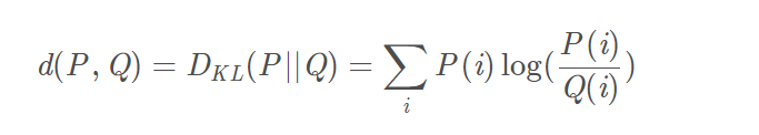
KL散度是一种概率分布和另一种概率分布的差异的距离。
公式如下：

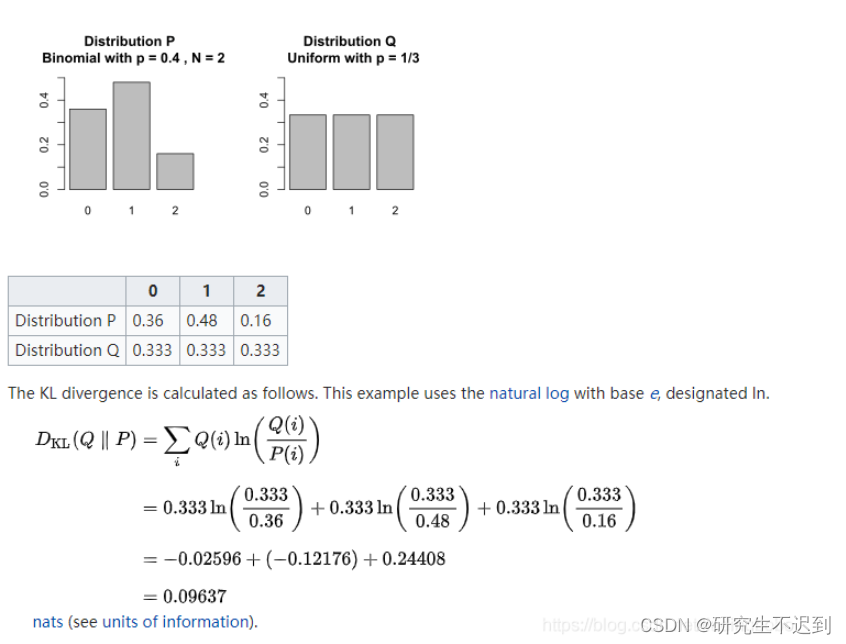
2 一个简单的例子

3 KL的性质

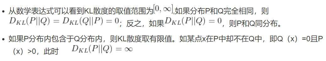
1. 具有非对称性，且不满足三角不等式形式，即是$D_{KL}(P||Q)\ne D_{KL}(Q||P)$，说明KL散度不是用来衡量距离的。
2. 如图：

4 KL散度的公式介绍

公式如下：

其中，$D_{KL}(P||Q)$——概率$P$与概率$Q$之间的差异，散度越小，则两个概率越接近，那么估计的概率分布也就与真实的概率分布越接近。

KL散度，计算出来的是两者的概率差，可以说KL散度是一种损失，来计算两者的概率差异。

5 Pytorch实现KL散度——F.kl_div()

5.1 函数原型

torch.nn.functional.kl_div(input, target, size_average=None, reduce=None, reduction='mean')

• 参数介绍：

input – Tensor of arbitrary shape

target – Tensor of the same shape as input

size_average (bool, optional) – Deprecated (see reduction). By default, the losses are averaged over each loss element in the batch. Note that for some losses, there multiple elements per sample. If the field size_average is set to False, the losses are instead summed for each minibatch. Ignored when reduce is False. Default: True

reduce (bool, optional) – Deprecated (see reduction). By default, the losses are averaged or summed over observations for each minibatch depending on size_average. When reduce is False, returns a loss per batch element instead and ignores size_average. Default: True

reduction (string, optional) – Specifies the reduction to apply to the output: 'none' | 'batchmean' | 'sum' | 'mean'. 'none': no reduction will be applied 'batchmean': the sum of the output will be divided by the batchsize 'sum': the output will be summed 'mean': the output will be divided by the number of elements in the output Default: 'mean'
{'none' | 'batchmean' | 'sum' | 'mean'}
'none':不进行压缩
'batchmean':输出的总和除以batchsize 
'sum':输出的总和
'mean':输出的输出除以输出中的元素数量
默认值：'mean'

1. 第一个参数是一个对数概率矩阵，第二个参数是概率矩阵。这里很重要，不然求出来的kl散度可能是个负值。

2. 如果现在想用Y指导X，第一个参数要传X，第二个要传Y。就是被指导的放在前面，然后求相应的概率和对数概率就可以了。例如$D_{KL}(P||Q)$，就是求Q的对数概率，求P的概率。

3. reduce bool类型，可选{‘True’, ‘False’}，默认值：TRUE.
   默认情况下，根据大小的平均值，对每个小批处理的损失进行平均或求和。当reduce为False时，返回每个批元素的损失值，并忽略平均大小。

4. reduction string类型，可选{‘None’, ‘batchmean’, ‘sum’, ‘mean’}，默认值：‘mean’
   ‘none’:不进行压缩
   ‘batchmean’:输出的总和除以batchsize
   ‘sum’:输出的总和
   ‘mean’:输出的输出除以输出中的元素数量

5.2 简单代码

import torch
import torch.nn.functional as F

# 定义两个矩阵
P = torch.tensor([0.25] * 4 + [0])
Q = torch.tensor([0.2] * 5)

print(P, Q)

# 因为要用P指导Q,所以求Q的对数概率，P的概率
log_Q = F.log_softmax(P, dim=-1)
_P = F.softmax(Q, dim=-1)

kl_sum = F.kl_div(log_Q, _P, reduction='sum')

print("SUM:", kl_sum)

-输出如下：

tensor([0.2500, 0.2500, 0.2500, 0.2500, 0.0000]) tensor([0.2000, 0.2000, 0.2000, 0.2000, 0.2000])
SUM: tensor(0.2231)

6 KL散度在R- Drop中的应用

6.1 什么是Dropout?

• 下面这篇文章我已经详细介绍过了，感兴趣的小伙伴可以移步下方链接：

https://blog.csdn.net/weixin_42521185/article/details/124359544

• Dropout的使用场景一般是神经元较多的神经网络，因为神经元较多可能会使得预测结果过拟合，采用Dropout随机丢弃一些神经元，可以很好的处理这个问题。

• 但是，Dropout的缺点也很明显：dropout是随机丢弃，所以训练和预测阶段使用的神经网络不同！

6.2 引入 R-drop

• step1：首先计算$L_{LK}$。
  不同模型训练经过不同的dropout可能会产生较大的差异，而我们这里通过KL散度将这些差异缩小，从而能够达到预测较准的情况。
  
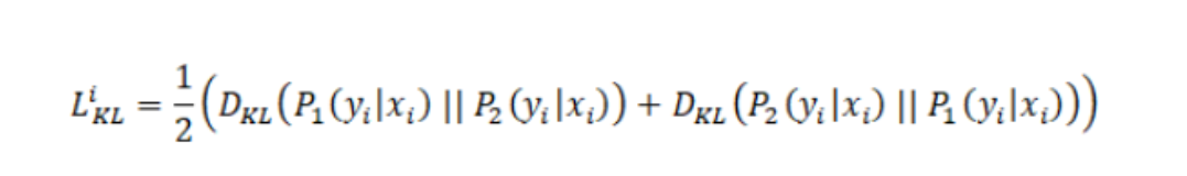
• step2：新的损失函数
  

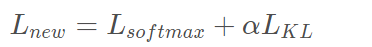
6.3 在R-Drop的代码

from tensorflow.keras.losses import kullback_leibler_divergence as kld
def categorical_crossentropy_with_rdrop(y_true, y_pred,alpha=1):
    """配合上述生成器的R-Drop Loss
    其实loss_kl的除以4，是为了在数量上对齐公式描述结果。
    """
    loss_ce = K.sparse_categorical_crossentropy(y_true, y_pred)  # 原来的loss
    #这里调用K.Sparse，一部分是常规的交叉熵
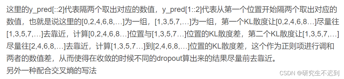
    loss_kl = kld(y_pred[::2], y_pred[1::2]) + kld(y_pred[1::2], y_pred[::2])
    #另一部分是两个模型的对称KL散度
    return K.mean(loss_ce) + K.mean(loss_kl) / 4 * alpha

• step1 首先调用交叉熵损失函数。

loss_ce = K.sparse_categorical_crossentropy(y_true,y_pred)

• step2 然后调用KL散度的内容

这里参考“唐僧爱吃唐僧肉的解释”

• 本研究生已疲惫了…