高光谱图像分类

1.简介

本文是根据论文《HybridSN: Exploring 3-D–2-DCNN Feature Hierarchy for Hyperspectral Image Classification》进行编写的。
高光谱图像分类在遥感图像分析中得到了广泛的应用。高光谱图像包括不同波段的图像。卷积神经网络(CNN)是最常用的基于深度学习的视觉数据处理方法之一。在最近的网络架构中也可以看到使用CNN进行HSI分类。这些方法大多基于二维CNN。另一方面，HSI分类性能高度依赖于空间和光谱信息。由于增加了计算的复杂性，很少有方法使用3d - cnn。总的来说，HybridSN是一个光谱空间3-DCNN，然后是空间2-D-CNN。3-D-CNN促进了光谱波段叠加的联合空间光谱特征表示。在三维cnn之上的二维cnn进一步学习更抽象的空间表示。此外，与单独使用三维cnn相比，混合cnn的使用降低了模型的复杂性。为此，作者提出了HybridSN 模型：混合特征学习框架。

2.HybridSN 模型

HybridSN 模型：混合特征学习框架（hybrid feature learning framework）
网络结构如图所示（三个三维卷积，一个二维卷积，三个全连接层）：

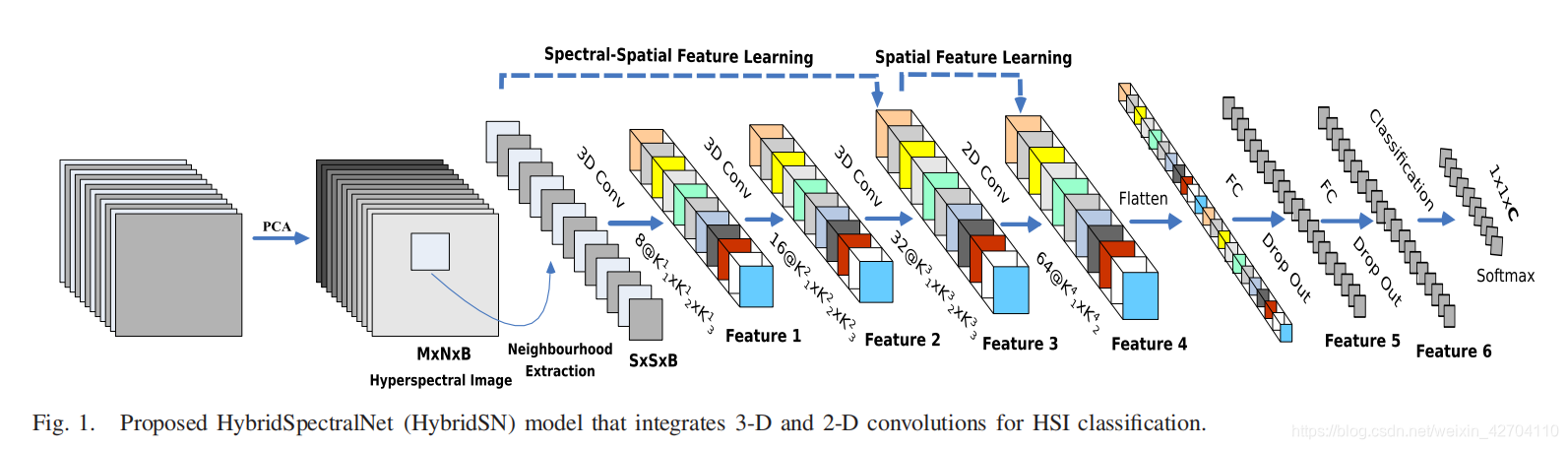
三维卷积中，卷积核的尺寸为8×3×3×7×1、16×3×3×5×8、32×3×3×3×16（16个三维核，3×3×5维）
二维卷积中，卷积核的尺寸为64×3×3×576（576为二维输入特征图的数量）

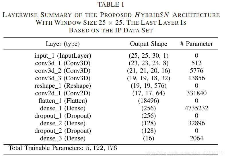
下面是HybridSN网络层数结构表：

3.具体代码实现

环境：谷歌colab+pytorch

3.1首先取得数据，并引入基本函数库

! wget http://www.ehu.eus/ccwintco/uploads/6/67/Indian_pines_corrected.mat
! wget http://www.ehu.eus/ccwintco/uploads/c/c4/Indian_pines_gt.mat
! pip install spectral

import numpy as np
import matplotlib.pyplot as plt
import scipy.io as sio
from sklearn.decomposition import PCA
from sklearn.model_selection import train_test_split
from sklearn.metrics import confusion_matrix, accuracy_score, classification_report, cohen_kappa_score
import spectral
import torch
import torchvision
import torch.nn as nn
import torch.nn.functional as F
import torch.optim as optim

3.2HybridSN 网络类的代码

class_num = 16

class HybridSN(nn.Module):
  def __init__(self):
    super(HybridSN, self).__init__()
    self.conv3d_1 = nn.Sequential(
        nn.Conv3d(1, 8, kernel_size=(7, 3, 3), stride=1, padding=0),
        nn.BatchNorm3d(8),
        nn.ReLU(inplace = True),
    )
    self.conv3d_2 = nn.Sequential(
        nn.Conv3d(8, 16, kernel_size=(5, 3, 3), stride=1, padding=0),
        nn.BatchNorm3d(16),
        nn.ReLU(inplace = True),
    ) 
    self.conv3d_3 = nn.Sequential(
        nn.Conv3d(16, 32, kernel_size=(3, 3, 3), stride=1, padding=0),
        nn.BatchNorm3d(32),
        nn.ReLU(inplace = True)
    )

    self.conv2d_4 = nn.Sequential(
        nn.Conv2d(576, 64, kernel_size=(3, 3), stride=1, padding=0),
        nn.BatchNorm2d(64),
        nn.ReLU(inplace = True),
    )
    self.fc1 = nn.Linear(18496,256)
    self.fc2 = nn.Linear(256,128)
    self.fc3 = nn.Linear(128,16)
    self.dropout = nn.Dropout(p = 0.4)

  def forward(self,x):
    out = self.conv3d_1(x)
    out = self.conv3d_2(out)
    out = self.conv3d_3(out)
    out = self.conv2d_4(out.reshape(out.shape[0],-1,19,19))
    out = out.reshape(out.shape[0],-1)
    out = F.relu(self.dropout(self.fc1(out)))
    out = F.relu(self.dropout(self.fc2(out)))
    out = self.fc3(out)
    return out

3.3 定义基本函数

首先对高光谱数据实施PCA降维；然后创建 keras 方便处理的数据格式；然后随机抽取 10% 数据做为训练集，剩余的做为测试集。

# 对高光谱数据 X 应用 PCA 变换
def applyPCA(X, numComponents):
    newX = np.reshape(X, (-1, X.shape[2]))
    pca = PCA(n_components=numComponents, whiten=True)
    newX = pca.fit_transform(newX)
    newX = np.reshape(newX, (X.shape[0], X.shape[1], numComponents))
    return newX

# 对单个像素周围提取 patch 时，边缘像素就无法取了，因此，给这部分像素进行 padding 操作
def padWithZeros(X, margin=2):
    newX = np.zeros((X.shape[0] + 2 * margin, X.shape[1] + 2* margin, X.shape[2]))
    x_offset = margin
    y_offset = margin
    newX[x_offset:X.shape[0] + x_offset, y_offset:X.shape[1] + y_offset, :] = X
    return newX

# 在每个像素周围提取 patch ，然后创建成符合 keras 处理的格式
def createImageCubes(X, y, windowSize=5, removeZeroLabels = True):
    # 给 X 做 padding
    margin = int((windowSize - 1) / 2)
    zeroPaddedX = padWithZeros(X, margin=margin)
    # split patches
    patchesData = np.zeros((X.shape[0] * X.shape[1], windowSize, windowSize, X.shape[2]))
    patchesLabels = np.zeros((X.shape[0] * X.shape[1]))
    patchIndex = 0
    for r in range(margin, zeroPaddedX.shape[0] - margin):
        for c in range(margin, zeroPaddedX.shape[1] - margin):
            patch = zeroPaddedX[r - margin:r + margin + 1, c - margin:c + margin + 1]   
            patchesData[patchIndex, :, :, :] = patch
            patchesLabels[patchIndex] = y[r-margin, c-margin]
            patchIndex = patchIndex + 1
    if removeZeroLabels:
        patchesData = patchesData[patchesLabels>0,:,:,:]
        patchesLabels = patchesLabels[patchesLabels>0]
        patchesLabels -= 1
    return patchesData, patchesLabels

def splitTrainTestSet(X, y, testRatio, randomState=345):
    X_train, X_test, y_train, y_test = train_test_split(X, y, test_size=testRatio, random_state=randomState, stratify=y)
    return X_train, X_test, y_train, y_test

3.4读取并创建数据集

# 地物类别
class_num = 16
X = sio.loadmat('Indian_pines_corrected.mat')['indian_pines_corrected']
y = sio.loadmat('Indian_pines_gt.mat')['indian_pines_gt']

# 用于测试样本的比例
test_ratio = 0.90
# 每个像素周围提取 patch 的尺寸
patch_size = 25
# 使用 PCA 降维，得到主成分的数量
pca_components = 30

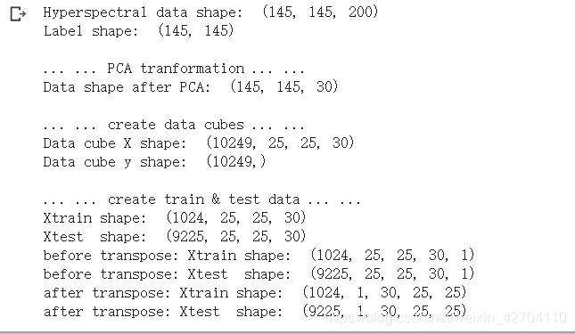
print('Hyperspectral data shape: ', X.shape)
print('Label shape: ', y.shape)

print('\n... ... PCA tranformation ... ...')
X_pca = applyPCA(X, numComponents=pca_components)
print('Data shape after PCA: ', X_pca.shape)

print('\n... ... create data cubes ... ...')
X_pca, y = createImageCubes(X_pca, y, windowSize=patch_size)
print('Data cube X shape: ', X_pca.shape)
print('Data cube y shape: ', y.shape)

print('\n... ... create train & test data ... ...')
Xtrain, Xtest, ytrain, ytest = splitTrainTestSet(X_pca, y, test_ratio)
print('Xtrain shape: ', Xtrain.shape)
print('Xtest  shape: ', Xtest.shape)

# 改变 Xtrain, Ytrain 的形状，以符合 keras 的要求
Xtrain = Xtrain.reshape(-1, patch_size, patch_size, pca_components, 1)
Xtest  = Xtest.reshape(-1, patch_size, patch_size, pca_components, 1)
print('before transpose: Xtrain shape: ', Xtrain.shape) 
print('before transpose: Xtest  shape: ', Xtest.shape) 

# 为了适应 pytorch 结构，数据要做 transpose
Xtrain = Xtrain.transpose(0, 4, 3, 1, 2)
Xtest  = Xtest.transpose(0, 4, 3, 1, 2)
print('after transpose: Xtrain shape: ', Xtrain.shape) 
print('after transpose: Xtest  shape: ', Xtest.shape) 


""" Training dataset"""
class TrainDS(torch.utils.data.Dataset): 
    def __init__(self):
        self.len = Xtrain.shape[0]
        self.x_data = torch.FloatTensor(Xtrain)
        self.y_data = torch.LongTensor(ytrain)        
    def __getitem__(self, index):
        # 根据索引返回数据和对应的标签
        return self.x_data[index], self.y_data[index]
    def __len__(self): 
        # 返回文件数据的数目
        return self.len

""" Testing dataset"""
class TestDS(torch.utils.data.Dataset): 
    def __init__(self):
        self.len = Xtest.shape[0]
        self.x_data = torch.FloatTensor(Xtest)
        self.y_data = torch.LongTensor(ytest)
    def __getitem__(self, index):
        # 根据索引返回数据和对应的标签
        return self.x_data[index], self.y_data[index]
    def __len__(self): 
        # 返回文件数据的数目
        return self.len

# 创建 trainloader 和 testloader
trainset = TrainDS()
testset  = TestDS()
train_loader = torch.utils.data.DataLoader(dataset=trainset, batch_size=128, shuffle=True, num_workers=2)
test_loader  = torch.utils.data.DataLoader(dataset=testset,  batch_size=128, shuffle=False, num_workers=2)

3.5 开始训练

# 使用GPU训练，可以在菜单 "代码执行工具" -> "更改运行时类型" 里进行设置
device = torch.device("cuda:0" if torch.cuda.is_available() else "cpu")

# 网络放到GPU上
net = HybridSN().to(device)
criterion = nn.CrossEntropyLoss()
optimizer = optim.Adam(net.parameters(), lr=0.001)

# 开始训练
total_loss = 0
for epoch in range(100):
    for i, (inputs, labels) in enumerate(train_loader):
        inputs = inputs.to(device)
        labels = labels.to(device)
        # 优化器梯度归零
        optimizer.zero_grad()
        # 正向传播 +　反向传播 + 优化 
        outputs = net(inputs)
        loss = criterion(outputs, labels)
        loss.backward()
        optimizer.step()
        total_loss += loss.item()
    print('[Epoch: %d]   [loss avg: %.4f]   [current loss: %.4f]' %(epoch + 1, total_loss/(epoch+1), loss.item()))

print('Finished Training')

训练结果：
[Epoch: 1] [loss avg: 21.4777] [current loss: 2.1179]
[Epoch: 2] [loss avg: 17.9520] [current loss: 1.4763]
[Epoch: 3] [loss avg: 15.8319] [current loss: 1.3697]
[Epoch: 4] [loss avg: 14.2346] [current loss: 0.9965]
[Epoch: 5] [loss avg: 12.8106] [current loss: 0.7685]
[Epoch: 6] [loss avg: 11.5739] [current loss: 0.5164]
[Epoch: 7] [loss avg: 10.4780] [current loss: 0.5538]
[Epoch: 8] [loss avg: 9.5241] [current loss: 0.2097]
[Epoch: 9] [loss avg: 8.6989] [current loss: 0.1793]
[Epoch: 10] [loss avg: 7.9854] [current loss: 0.3112]
[Epoch: 11] [loss avg: 7.3737] [current loss: 0.2170]
[Epoch: 12] [loss avg: 6.8384] [current loss: 0.1424]
[Epoch: 13] [loss avg: 6.3778] [current loss: 0.1558]
[Epoch: 14] [loss avg: 5.9814] [current loss: 0.1140]
[Epoch: 15] [loss avg: 5.6361] [current loss: 0.0886]
[Epoch: 16] [loss avg: 5.3210] [current loss: 0.0716]
[Epoch: 17] [loss avg: 5.0419] [current loss: 0.0531]
[Epoch: 18] [loss avg: 4.7874] [current loss: 0.0812]
[Epoch: 19] [loss avg: 4.5536] [current loss: 0.0947]
[Epoch: 20] [loss avg: 4.3511] [current loss: 0.0338]
[Epoch: 21] [loss avg: 4.1675] [current loss: 0.0848]
[Epoch: 22] [loss avg: 3.9951] [current loss: 0.0782]
[Epoch: 23] [loss avg: 3.8362] [current loss: 0.0718]
[Epoch: 24] [loss avg: 3.6959] [current loss: 0.0472]
[Epoch: 25] [loss avg: 3.5727] [current loss: 0.0677]
[Epoch: 26] [loss avg: 3.4577] [current loss: 0.1050]
[Epoch: 27] [loss avg: 3.3503] [current loss: 0.1232]
[Epoch: 28] [loss avg: 3.2424] [current loss: 0.0768]
[Epoch: 29] [loss avg: 3.1380] [current loss: 0.0425]
[Epoch: 30] [loss avg: 3.0444] [current loss: 0.0410]
[Epoch: 31] [loss avg: 2.9534] [current loss: 0.0108]
[Epoch: 32] [loss avg: 2.8671] [current loss: 0.0374]
[Epoch: 33] [loss avg: 2.7853] [current loss: 0.0141]
[Epoch: 34] [loss avg: 2.7086] [current loss: 0.0306]
[Epoch: 35] [loss avg: 2.6346] [current loss: 0.0028]
[Epoch: 36] [loss avg: 2.5678] [current loss: 0.0113]
[Epoch: 37] [loss avg: 2.5009] [current loss: 0.0187]
[Epoch: 38] [loss avg: 2.4391] [current loss: 0.0111]
[Epoch: 39] [loss avg: 2.3793] [current loss: 0.0137]
[Epoch: 40] [loss avg: 2.3257] [current loss: 0.0229]
[Epoch: 41] [loss avg: 2.2726] [current loss: 0.0464]
[Epoch: 42] [loss avg: 2.2217] [current loss: 0.0231]
[Epoch: 43] [loss avg: 2.1736] [current loss: 0.0045]
[Epoch: 44] [loss avg: 2.1273] [current loss: 0.0253]
[Epoch: 45] [loss avg: 2.0834] [current loss: 0.0129]
[Epoch: 46] [loss avg: 2.0396] [current loss: 0.0145]
[Epoch: 47] [loss avg: 1.9989] [current loss: 0.0278]
[Epoch: 48] [loss avg: 1.9598] [current loss: 0.0080]
[Epoch: 49] [loss avg: 1.9226] [current loss: 0.0306]
[Epoch: 50] [loss avg: 1.8873] [current loss: 0.0212]
[Epoch: 51] [loss avg: 1.8540] [current loss: 0.0456]
[Epoch: 52] [loss avg: 1.8215] [current loss: 0.0104]
[Epoch: 53] [loss avg: 1.7902] [current loss: 0.1154]
[Epoch: 54] [loss avg: 1.7604] [current loss: 0.0005]
[Epoch: 55] [loss avg: 1.7315] [current loss: 0.0594]
[Epoch: 56] [loss avg: 1.7079] [current loss: 0.0063]
[Epoch: 57] [loss avg: 1.6874] [current loss: 0.0431]
[Epoch: 58] [loss avg: 1.6631] [current loss: 0.0191]
[Epoch: 59] [loss avg: 1.6390] [current loss: 0.0165]
[Epoch: 60] [loss avg: 1.6160] [current loss: 0.0346]
[Epoch: 61] [loss avg: 1.5916] [current loss: 0.0196]
[Epoch: 62] [loss avg: 1.5676] [current loss: 0.0131]
[Epoch: 63] [loss avg: 1.5464] [current loss: 0.0049]
[Epoch: 64] [loss avg: 1.5238] [current loss: 0.0007]
[Epoch: 65] [loss avg: 1.5026] [current loss: 0.0055]
[Epoch: 66] [loss avg: 1.4821] [current loss: 0.0173]
[Epoch: 67] [loss avg: 1.4629] [current loss: 0.0005]
[Epoch: 68] [loss avg: 1.4440] [current loss: 0.0413]
[Epoch: 69] [loss avg: 1.4256] [current loss: 0.0023]
[Epoch: 70] [loss avg: 1.4073] [current loss: 0.0021]
[Epoch: 71] [loss avg: 1.3918] [current loss: 0.0058]
[Epoch: 72] [loss avg: 1.3756] [current loss: 0.0167]
[Epoch: 73] [loss avg: 1.3605] [current loss: 0.0069]
[Epoch: 74] [loss avg: 1.3437] [current loss: 0.0128]
[Epoch: 75] [loss avg: 1.3268] [current loss: 0.0012]
[Epoch: 76] [loss avg: 1.3117] [current loss: 0.0037]
[Epoch: 77] [loss avg: 1.2965] [current loss: 0.0227]
[Epoch: 78] [loss avg: 1.2834] [current loss: 0.0376]
[Epoch: 79] [loss avg: 1.2688] [current loss: 0.0016]
[Epoch: 80] [loss avg: 1.2545] [current loss: 0.0041]
[Epoch: 81] [loss avg: 1.2414] [current loss: 0.0085]
[Epoch: 82] [loss avg: 1.2296] [current loss: 0.0122]
[Epoch: 83] [loss avg: 1.2165] [current loss: 0.0030]
[Epoch: 84] [loss avg: 1.2041] [current loss: 0.0033]
[Epoch: 85] [loss avg: 1.1913] [current loss: 0.0009]
[Epoch: 86] [loss avg: 1.1782] [current loss: 0.0067]
[Epoch: 87] [loss avg: 1.1651] [current loss: 0.0013]
[Epoch: 88] [loss avg: 1.1530] [current loss: 0.0046]
[Epoch: 89] [loss avg: 1.1406] [current loss: 0.0057]
[Epoch: 90] [loss avg: 1.1286] [current loss: 0.0060]
[Epoch: 91] [loss avg: 1.1172] [current loss: 0.0002]
[Epoch: 92] [loss avg: 1.1056] [current loss: 0.0056]
[Epoch: 93] [loss avg: 1.0954] [current loss: 0.0119]
[Epoch: 94] [loss avg: 1.0845] [current loss: 0.0121]
[Epoch: 95] [loss avg: 1.0743] [current loss: 0.0079]
[Epoch: 96] [loss avg: 1.0638] [current loss: 0.0249]
[Epoch: 97] [loss avg: 1.0536] [current loss: 0.0275]
[Epoch: 98] [loss avg: 1.0441] [current loss: 0.0512]
[Epoch: 99] [loss avg: 1.0359] [current loss: 0.0089]
[Epoch: 100] [loss avg: 1.0268] [current loss: 0.0043]
Finished Training

3.6 模型测试

count = 0
# 模型测试
for inputs, _ in test_loader:
    inputs = inputs.to(device)
    outputs = net(inputs)
    outputs = np.argmax(outputs.detach().cpu().numpy(), axis=1)
    if count == 0:
        y_pred_test =  outputs
        count = 1
    else:
        y_pred_test = np.concatenate( (y_pred_test, outputs) )

# 生成分类报告
classification = classification_report(ytest, y_pred_test, digits=4)
print(classification)

测试结果：

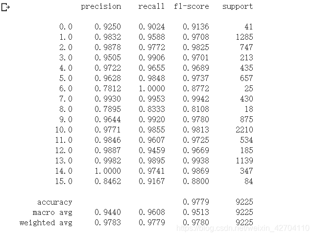
准确率为达到了97.79%

3.7 备用函数

下面是用于计算各个类准确率，显示结果的备用函数，以供参考

from operator import truediv

def AA_andEachClassAccuracy(confusion_matrix):
    counter = confusion_matrix.shape[0]
    list_diag = np.diag(confusion_matrix)
    list_raw_sum = np.sum(confusion_matrix, axis=1)
    each_acc = np.nan_to_num(truediv(list_diag, list_raw_sum))
    average_acc = np.mean(each_acc)
    return each_acc, average_acc


def reports (test_loader, y_test, name):
    count = 0
    # 模型测试
    for inputs, _ in test_loader:
        inputs = inputs.to(device)
        outputs = net(inputs)
        outputs = np.argmax(outputs.detach().cpu().numpy(), axis=1)
        if count == 0:
            y_pred =  outputs
            count = 1
        else:
            y_pred = np.concatenate( (y_pred, outputs) )

    if name == 'IP':
        target_names = ['Alfalfa', 'Corn-notill', 'Corn-mintill', 'Corn'
                        ,'Grass-pasture', 'Grass-trees', 'Grass-pasture-mowed', 
                        'Hay-windrowed', 'Oats', 'Soybean-notill', 'Soybean-mintill',
                        'Soybean-clean', 'Wheat', 'Woods', 'Buildings-Grass-Trees-Drives',
                        'Stone-Steel-Towers']
    elif name == 'SA':
        target_names = ['Brocoli_green_weeds_1','Brocoli_green_weeds_2','Fallow','Fallow_rough_plow','Fallow_smooth',
                        'Stubble','Celery','Grapes_untrained','Soil_vinyard_develop','Corn_senesced_green_weeds',
                        'Lettuce_romaine_4wk','Lettuce_romaine_5wk','Lettuce_romaine_6wk','Lettuce_romaine_7wk',
                        'Vinyard_untrained','Vinyard_vertical_trellis']
    elif name == 'PU':
        target_names = ['Asphalt','Meadows','Gravel','Trees', 'Painted metal sheets','Bare Soil','Bitumen',
                        'Self-Blocking Bricks','Shadows']
    
    classification = classification_report(y_test, y_pred, target_names=target_names)
    oa = accuracy_score(y_test, y_pred)
    confusion = confusion_matrix(y_test, y_pred)
    each_acc, aa = AA_andEachClassAccuracy(confusion)
    kappa = cohen_kappa_score(y_test, y_pred)
    
    return classification, confusion, oa*100, each_acc*100, aa*100, kappa*100

检测结果写在文件里：

classification, confusion, oa, each_acc, aa, kappa = reports(test_loader, ytest, 'IP')
classification = str(classification)
confusion = str(confusion)
file_name = "classification_report.txt"

with open(file_name, 'w') as x_file:
    x_file.write('\n')
    x_file.write('{} Kappa accuracy (%)'.format(kappa))
    x_file.write('\n')
    x_file.write('{} Overall accuracy (%)'.format(oa))
    x_file.write('\n')
    x_file.write('{} Average accuracy (%)'.format(aa))
    x_file.write('\n')
    x_file.write('\n')
    x_file.write('{}'.format(classification))
    x_file.write('\n')
    x_file.write('{}'.format(confusion))

下面代码用于显示分类结果：

# load the original image
X = sio.loadmat('Indian_pines_corrected.mat')['indian_pines_corrected']
y = sio.loadmat('Indian_pines_gt.mat')['indian_pines_gt']

height = y.shape[0]
width = y.shape[1]

X = applyPCA(X, numComponents= pca_components)
X = padWithZeros(X, patch_size//2)

# 逐像素预测类别
outputs = np.zeros((height,width))
for i in range(height):
    for j in range(width):
        if int(y[i,j]) == 0:
            continue
        else :
            image_patch = X[i:i+patch_size, j:j+patch_size, :]
            image_patch = image_patch.reshape(1,image_patch.shape[0],image_patch.shape[1], image_patch.shape[2], 1)
            X_test_image = torch.FloatTensor(image_patch.transpose(0, 4, 3, 1, 2)).to(device)                                   
            prediction = net(X_test_image)
            prediction = np.argmax(prediction.detach().cpu().numpy(), axis=1)
            outputs[i][j] = prediction+1
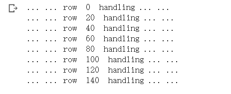
    if i % 20 == 0:
        print('... ... row ', i, ' handling ... ...')

predict_image = spectral.imshow(classes = outputs.astype(int),figsize =(5,5))

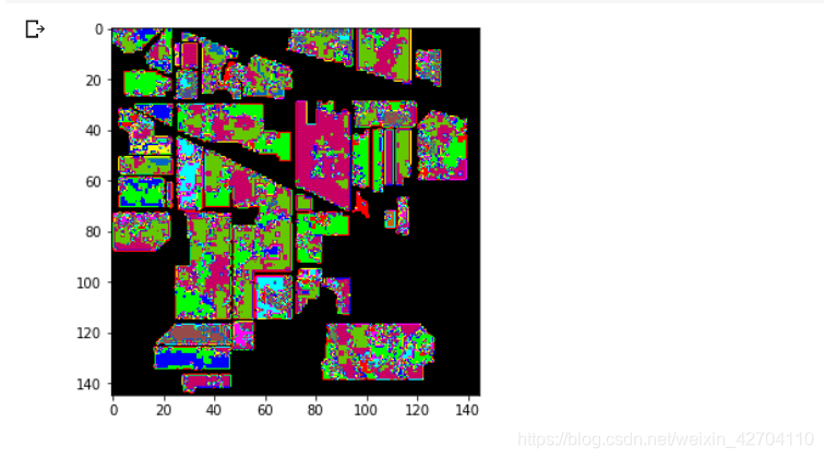
可以看到分类的结果并不是很理想。

4. 思考题

训练网络，然后多测试几次，会发现每次分类的结果都不一样，请思考为什么？
在model(test)之前，需要加上model.eval()，其作用是为了固定BN和dropout层，使得偏置参数不随着发生变化。否则的话，有输入数据，即使不训练，它也会改变权值。这是model中含有batch normalization层所带来的的性质。
BN的作用主要是对网络中间的每层进行归一化处理，并且使用变换重构（Batch Normalization Transform）保证每层提取的特征分布不会被破坏。
训练时是针对每个mini-batch的，但是测试是针对单张图片的，即不存在batch的概念。在做one classification的时候，训练集和测试集的样本分布是不一样的。
Dropout在train时随机选择神经元而predict要使用全部神经元并且要乘一个补偿系数。
BN在train时每个batch做了不同的归一化因此也对应了不同的参数，相应predict时实际用的参数是每个batch下参数的移动平均。

思考问题，如果想要进一步提升高光谱图像的分类性能，可以如何使用注意力机制？
注意力机制最早用于NLP，后来在计算机视觉领域（CV）种也得到广泛应用，注意力机制被引入来进行视觉信息处理。注意力机制没有严格的数学定义，列如传统的局部图像特征提取，滑动窗口方法等可以看作是一种注意力机制。在神经网络中，注意力机制通常是一种额外的神经网络，能够硬性选择输入的某些部分，或者给输入的不同部分分配不同的权重。注意力机制能够从大量信息中筛选出重要的信息。
在神经网络中引入注意力机制有很多方法，以卷积审计网络为例，可以在空间维度增加引入attention机制，也可以在通道维度（channel）增加attention机制，当然也有混合维度即同时在空间维度和通道维度增加attention机制。

可以利用**SENet（Squeeze-and-Excitation Network）**进一步提升高光谱图像的分类性能，SENet在通道维度（channel）上增加attention机制。

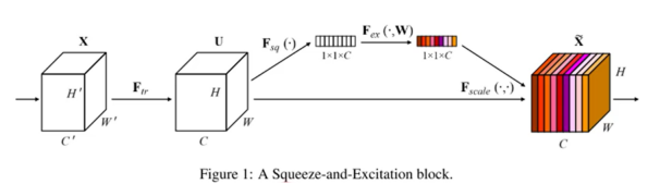
SENet在通道维度（channel）上增加attention机制，关键的两个操作是Squeeze(压缩)和Excitation(激发)，这个attention结构命名为SE block，SE block通过自动学习的方式获取到每个特征通道的重要程度，然后用这个重要程度去给每个特征通道赋予一个权重值，从而让神经网络重点关注这些特征通道，即提升对当前任务有用的特征通道并抑制对当前任务用处不大的特征通道。
SE模块实现的 Pytorch版:

class SELayer(nn.Module):
    def __init__(self, channel, reduction=16):
        super(SELayer, self).__init__()
        self.avg_pool = nn.AdaptiveAvgPool2d(1)
        self.fc = nn.Sequential(
            nn.Linear(channel, channel // reduction, bias=False),
            nn.ReLU(inplace=True),
            nn.Linear(channel // reduction, channel, bias=False),
            nn.Sigmoid()
        )

    def forward(self, x):
        b, c, _, _ = x.size()
        y = self.avg_pool(x).view(b, c)
        y = self.fc(y).view(b, c, 1, 1)
        return x * y.expand_as(x)

参考：
https://blog.csdn.net/weixin_42907473/article/details/106525668?utm_medium=distribute.pc_relevant.none-task-blog-searchFromBaidu-2.control&depth_1-utm_source=distribute.pc_relevant.none-task-blog-searchFromBaidu-2.control
https://www.bilibili.com/video/BV1SA41147uA?from=search&seid=15297804892011941113