【数学建模】进化计算与群体智能

最新推荐文章于 2024-07-20 17:16:00 发布

宏辉

最新推荐文章于 2024-07-20 17:16:00 发布

阅读量702

点赞数 20

分类专栏：数学建模文章标签：数学建模算法

本文链接：https://blog.csdn.net/weixin_42914989/article/details/140088875

版权

数学建模专栏收录该内容

6 篇文章 0 订阅

订阅专栏

进化计算与群体智能

1. 遗传算法理论与实现

1.1 遗传算法介绍

遗传算法（GA）是一种用于优化和搜索问题的启发式算法。它模拟了自然选择的过程，其中个体通过遗传和变异进行繁殖，逐渐进化出更优的解。

基本步骤：

初始化：生成初始种群。
适应度评估：评估种群中每个个体的适应度。
选择：根据适应度选择个体进行繁殖。
交叉：选定个体对进行基因交换，生成新的后代。
变异：对一些个体进行基因变异，以增加多样性。
迭代：重复评估和繁殖过程，直至达到停止条件。

1.2 遗传算法详细示例流程

目标是最大化函数 $f(x) = x^2$ ，其中 (x) 在区间 $[0, 31]$ 内，二进制编码为 5 位。

1) 初始种群

个体 A: 10101 (21)
个体 B: 11100 (28)
个体 C: 00011 (3)
个体 D: 01010 (10)

2) 适应度评估

计算每个个体的适应度 $f(x) = x^2$ ：

A: $f (21) = 441$
B: $f (28) = 784$
C: $f (3) = 9$
D: $f (10) = 100$

3) 选择（轮盘赌法）

计算适应度的总和： $441 + 784 + 9 + 100 = 1334$ 。

计算每个个体的选择概率：

A: $\approx 0.33$
B: $\approx 0.59$
C: $\approx 0.007$
D: $\approx 0.075$

累积概率分布：

A: 0.33
B: 0.33 + 0.59 = 0.92
C: 0.92 + 0.007 = 0.927
D: 0.927 + 0.075 = 1.0

通过轮盘赌法选择父代（假设随机数生成 0.4 和 0.7）：

0.4 落在 B 区间，选择 B。
0.7 落在 B 区间，再次选择 B。

假设再随机生成 0.1 和 0.95：

0.1 落在 A 区间，选择 A。
0.95 落在 D 区间，选择 D。

选出的父代：B (11100)、B (11100)、A (10101)、D (01010)

4) 交叉

选择交叉点（假设在第 3 位,那么会交换第3位后的基因）：

B (11100) 和 A (10101):
子代 1: 11101 (29)
子代 2: 10100 (20)
B (11100) 和 D (01010):
子代 3: 11110 (30)
子代 4: 01000 (8)

5) 变异

假设变异概率为 0.1（10%），对每个子代随机选择基因进行变异：

子代 1 (11101): 第 2 位变异 -> 10101 (21)
子代 2 (10100): 第 4 位变异 -> 10110 (22)
子代 3 (11110): 无变异 -> 11110 (30)
子代 4 (01000): 第 1 位变异 -> 11000 (24)

新的种群为：

个体 1: 10101 (21)
个体 2: 10110 (22)
个体 3: 11110 (30)
个体 4: 11000 (24)

6) 迭代

重复适应度评估、选择、交叉和变异步骤，直至达到停止条件（如最大代数或适应度不再提高）。

1.3 遗传算法的实现

在此给出最大化函数 $f(x) = x^2$ ，其中 (x) 在区间 $[0, 31]$ 内，二进制编码为 5 位的解题代码

import numpy as np

# 定义适应度函数
def fitness_function(x):
    return x**2

# 遗传算法的实现
def genetic_algorithm(num_generations, population_size, crossover_rate, mutation_rate):
    # 初始化种群
    population = np.random.randint(0, 32, size=(population_size, 1))  # 初始种群为整数编码，范围在[0, 31]之间
    
    for generation in range(num_generations):
        # 计算适应度
        fitness = np.array([fitness_function(x) for x in population[:, 0]])
        
        # 选择父代
        parents = select_parents(population, fitness)
        
        # 交叉
        offspring_crossover = crossover(parents, crossover_rate)
        
        # 变异
        offspring_mutation = mutate(offspring_crossover, mutation_rate)
        
        # 更新种群
        population = np.vstack((parents, offspring_mutation))
        
    # 返回最佳个体和最佳适应度
    best_index = np.argmax(fitness)
    best_individual = population[best_index][0]
    best_fitness = fitness[best_index]
    
    return best_individual, best_fitness

# 选择父代的方法（轮盘赌选择）
def select_parents(population, fitness):
    total_fitness = np.sum(fitness)
    probabilities = fitness / total_fitness
    parent_indices = np.random.choice(len(population), size=len(population), replace=True, p=probabilities)
    parents = population[parent_indices]
    return parents

# 交叉操作（单点交叉）
def crossover(parents, crossover_rate):
    offspring = np.empty_like(parents)
    for i in range(len(parents)//2):
        parent1 = parents[i]
        parent2 = parents[len(parents)-1-i]
        if np.random.rand() < crossover_rate:
            crossover_point = np.random.randint(0, len(parent1))
            offspring[i] = np.concatenate((parent1[:crossover_point], parent2[crossover_point:]))
            offspring[len(parents)-1-i] = np.concatenate((parent2[:crossover_point], parent1[crossover_point:]))
        else:
            offspring[i] = parent1
            offspring[len(parents)-1-i] = parent2
    return offspring

# 变异操作（单点变异）
def mutate(offspring, mutation_rate):
    for i in range(len(offspring)):
        if np.random.rand() < mutation_rate:
            mutation_point = np.random.randint(0, len(offspring[i]))
            offspring[i][mutation_point] = np.random.randint(0, 32)  # 重新随机生成一个值
    return offspring

# 示例参数
num_generations = 100
population_size = 50
crossover_rate = 0.8
mutation_rate = 0.01

# 运行遗传算法
best_individual, best_fitness = genetic_algorithm(num_generations, population_size, crossover_rate, mutation_rate)

print("最佳个体：", best_individual)
print("最佳适应度：", best_fitness)

1.4 scikit-opt 库实现遗传算法

安装库

首先，确保安装了 scikit-opt：

pip install scikit-opt

1.4.1 求解函数极值

要使用 scikit-opt 库中的遗传算法求解函数 $F(x, y) = x^2 + y^2 + \sin(x) + (1 - 0.001)x^2$ 的极值，可以按照以下步骤进行：

代码实现

import numpy as np
import matplotlib.pyplot as plt
from sko.GA import GA

# 定义目标函数
def objective_function(x):
    x1, x2 = x
    return x1**2 + x2**2 + np.sin(x1) + (1 - 0.001) * x1**2

# 设置遗传算法参数
ga = GA(func=objective_function, n_dim=2, size_pop=50, max_iter=200, lb=[-10, -10], ub=[10, 10], precision=1e-7)

# 运行遗传算法
best_x, best_y = ga.run()

# 打印结果
print(f"最佳解：x = {best_x}, y = {best_y}")

# 绘制损失函数迭代过程
plt.plot(ga.all_history_Y)
plt.title('迭代过程中的损失函数')
plt.xlabel('迭代次数')
plt.ylabel('损失函数值')
plt.show()

代码说明

目标函数：定义要优化的函数 $F(x, y) $。
遗传算法设置：
- n_dim=2 表示有两个变量 $x$ 和 $y$ 。
- size_pop=50 为种群规模。
- max_iter=200 为最大迭代次数。
- lb 和 ub 分别为变量的下界和上界。
运行算法：调用 run 方法执行遗传算法。
结果可视化：绘制损失函数随迭代次数的变化曲线。

运行结果

运行上述代码后，将得到最佳解和对应的损失函数值，并显示迭代过程中损失函数值的变化曲线。这样可以直观地看到遗传算法的收敛过程。

1.4.2 求解TSP 问题

在 sko 中，有专门用于解决 TSP 问题的接口 GA_TSP 来通过遗传算法解决 TSP 问题在这里插入图片描述

代码实现

import numpy as np
import matplotlib.pyplot as plt
from scipy.spatial import distance
from sko.GA import GA_TSP

def test2():
    num_points = 50
    points_coordinate = np.random.rand(num_points, 2)  # generate coordinate of points
    distance_matrix = distance.cdist(points_coordinate, points_coordinate, metric='euclidean')

    def cal_total_distance(routine):
        '''The objective function. input routine, return total distance.'''
        return sum(distance_matrix[routine[i], routine[(i + 1) % num_points]] for i in range(num_points))

    ga_tsp = GA_TSP(func=cal_total_distance, n_dim=num_points, size_pop=50, max_iter=500, prob_mut=1)
    best_points, best_distance = ga_tsp.run()
    fig, ax = plt.subplots(1, 2)
    best_points_ = np.concatenate([best_points, [best_points[0]]])
    best_points_coordinate = points_coordinate[best_points_, :]
    ax[0].plot(best_points_coordinate[:, 0], best_points_coordinate[:, 1], 'o-r')
    ax[1].plot(ga_tsp.generation_best_Y)
    plt.show()

代码说明

points_coordinate：创建城市坐标
dist_matrix：计算举例矩阵
GA_TSP：调用GA_TSP方法进行求解问题

运行结果

在这里插入图片描述

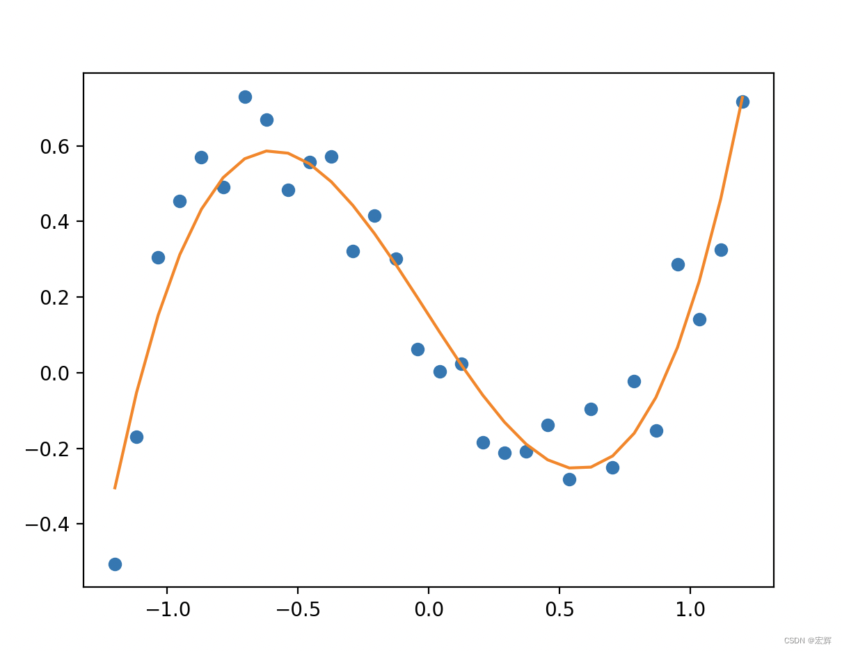
1.4.2 拟合数据

已知一组数据作坐标点，需要拟合出一元三次方程的系数。

设方程为 $ax^3+bx^2+cx+d$

代码实现

def test3():
    x_true = np.linspace(-1.2, 1.2, 30)
    y_true = x_true ** 3 - x_true + 0.4 * np.random.rand(30)
    plt.plot(x_true, y_true, 'o')

    def f_fun(x, a, b, c, d):
        return a * x ** 3 + b * x ** 2 + c * x + d

    def obj_fun(p):
        a, b, c, d = p
        residuals = np.square(f_fun(x_true, a, b, c, d) - y_true).sum()
        return residuals

    ga = GA(func=obj_fun, n_dim=4, size_pop=100, max_iter=500, lb=[-2] * 4, ub=[2] * 4)

    best_params, residuals = ga.run()
    print('best_x:', best_params, '\n', 'best_y:', residuals)
    y_predict = f_fun(x_true, *best_params)
    fig, ax = plt.subplots()
    ax.plot(x_true, y_true, 'o')
    ax.plot(x_true, y_predict, '-')
    plt.show()

运行结果

best_x: [ 1.04685973 0.04113689 -1.07711904 0.15250942] best_y: [0.37130528]
a = 1.04685973
b = 0.04113689
c = -1.07711904
d = 0.15250942
残差=0.37130528
绘制出曲线图如下图所示，数据点分布在拟合曲线的两侧。
在这里插入图片描述

2. 粒子群的理论与实现

2.1 粒子群算法介绍

粒子群优化算法（PSO）是一种基于群体智能的优化算法，由Kennedy和Eberhart于1995年提出。其灵感来源于鸟群觅食的行为。PSO通过在解空间中移动一群“粒子”来寻找最优解。每个粒子代表一个可能的解，并具有位置和速度。算法通过更新每个粒子的速度和位置，使其逐步接近最优解。

主要特点：

全局搜索能力强：粒子通过相互协作，避免陷入局部最优。
实现简单：参数较少，易于实现。

基本概念：

粒子位置：表示问题的一个解。
速度：决定粒子在搜索空间中的移动方向和步长。
个体最优位置（pbest）：粒子自身找到的最佳位置。
全局最优位置（gbest）：整个群体找到的最佳位置。

更新规则：

每个粒子根据自己的历史最佳位置（pbest）和群体历史最佳位置（gbest）调整速度和位置。

速度更新公式：
$v_{i} = w \cdot v_{i} + c_{1} \cdot r_{1} \cdot (pbest_{i} - x_{i}) + c_{2} \cdot r_{2} \cdot (gbest - x_{i})$

位置更新公式：
$x_{i} = x_{i} + v_{i}$

其中：

$w$ 是惯性权重，控制速度的影响。
$c_1, c_2$ 是学习因子，分别控制粒子对自身经验和群体经验的学习。
$r_1, r_2$ 是[0,1]的随机数。

2.2 粒子群算法的实现

以下是粒子群优化算法的Python实现，用于最大化函数 $f(x) = x^2$ 在区间 $[0, 31]$ 内：

import numpy as np

# 定义目标函数
def fitness_function(x):
    return x**2

# 粒子群优化算法实现
def particle_swarm_optimization(num_particles, num_iterations, w, c1, c2):
    # 初始化粒子的位置和速度
    positions = np.random.uniform(0, 31, (num_particles, 1))
    velocities = np.random.uniform(-1, 1, (num_particles, 1))
    
    # 初始化个体最佳位置和全局最佳位置
    pbest_positions = np.copy(positions)
    pbest_values = fitness_function(positions)
    gbest_position = pbest_positions[np.argmax(pbest_values)]
    gbest_value = np.max(pbest_values)
    
    for iteration in range(num_iterations):
        for i in range(num_particles):
            # 计算当前粒子的适应度
            fitness_value = fitness_function(positions[i])
            
            # 更新个体最佳位置
            if fitness_value > pbest_values[i]:
                pbest_values[i] = fitness_value
                pbest_positions[i] = positions[i]
        
        # 更新全局最佳位置
        if np.max(pbest_values) > gbest_value:
            gbest_value = np.max(pbest_values)
            gbest_position = pbest_positions[np.argmax(pbest_values)]
        
        # 更新粒子的速度和位置
        for i in range(num_particles):
            r1, r2 = np.random.rand(), np.random.rand()
            velocities[i] = (w * velocities[i] +
                             c1 * r1 * (pbest_positions[i] - positions[i]) +
                             c2 * r2 * (gbest_position - positions[i]))
            positions[i] += velocities[i]
        
        # 将位置限制在定义域内
        positions = np.clip(positions, 0, 31)
    
    return gbest_position, gbest_value

# 示例参数
num_particles = 30
num_iterations = 100
w = 0.5  # 惯性权重
c1 = 1.5  # 个体学习因子
c2 = 1.5  # 群体学习因子

# 运行粒子群优化算法
best_position, best_value = particle_swarm_optimization(num_particles, num_iterations, w, c1, c2)

print("最佳位置：", best_position)
print("最佳适应度：", best_value)

代码解释

初始化：
- 粒子位置和速度在指定范围内随机初始化。
个体最佳和全局最佳：
- 每个粒子维护其历史最佳位置（pbest）。
- 整个群体维护全局最佳位置（gbest）。
迭代过程：
- 每次迭代中，每个粒子根据自身和群体的历史信息更新速度和位置。
- 更新后的位置在定义域内进行裁剪。
返回结果：
- 最终返回找到的最佳位置和对应的适应度值。

现成的Python库可以用于粒子群优化。一个常用的库是 pyswarm。以下是使用 pyswarm 库求解 $f(x) = x^2$ 在区间 $[0, 31]$ 内的示例：

2.3 使用 `pyswarm` 进行粒子群算法求解

python库支持粒子群优化，如 pyswarm、 scipy（使用optimize.differential_evolution）和 pso 库。下面展示使用pyswarm进行求解。

安装 pyswarm：

如果还没有安装 pyswarm，可以通过以下命令安装：

pip install pyswarm

from pyswarm import pso

# 定义目标函数
def fitness_function(x):
    return -x**2  # 注意这里取负号，因为pyswarm默认是最小化

# 定义变量范围
lower_bound = [0]
upper_bound = [31]

# 使用pso进行优化
best_position, best_value = pso(fitness_function, lower_bound, upper_bound)

print("最佳位置：", best_position[0])
print("最佳适应度：", -best_value)  # 恢复原适应度

代码解释：

目标函数：目标函数定义为 $f(x) = -x^2$ 因为 pyswarm 默认最小化函数，所以对目标函数取负。
变量范围：定义搜索空间的上下界。
调用 pso 函数：pso 函数执行粒子群优化，返回最佳位置和适应度值。

3. 安利视频环节

学习本章推荐看b站有关遗传算法的介绍视频
遗传算法知识点＋例题讲解：通过例题超级详细讲解了遗传算法的各个步骤，强烈推荐看这个！！！

六分钟时间，带你走近遗传算法：TSP旅游商问题讲解，6分钟轻松拿下～

4. 一些知识点

4.1 遗传算法的编码和解码

编码长度的确定通常依赖于两个因素：值域的范围和所需的精度。具体步骤如下：

确定编码长度的步骤

确定值域范围：首先确定要编码的变量的取值范围，例如 $[a, b]$ 。
计算值域的宽度：计算值域的宽度 $W$ ，即 $W = b - a$ 。
确定精度：确定编码时希望达到的精度，如小数点后几位。
计算所需位数：根据精度和值域宽度计算所需的二进制位数 $L$ 。
- 如果精度为整数单位（如 1），则 $\lceil \log_2(W + 1) \rceil$ 。
- 如果精度不是整数单位（如 0.1、0.01 等），则 $\lceil \log_2\left(\frac{W}{d} + 1\right) \rceil$ ，其中 $d$ 是精度。

编码公式

计算编码长度：
$\lceil \log_2\left(\frac{b-a}{d}\right) \rceil$
$L$ 是编码所需的位数。
编码过程：
$binary_code = int ( x − a d ) \text{binary\_code} = \text{int}\left(\frac{x - a}{d}\right)$
将结果转为二进制字符串。

解码公式

解码过程：
$binary_code × d x = a + \text{binary\_code} \times d$

示例

假设区间 $[0, 10]$ ，精度 $d = 0.1$ ：

计算编码长度：
$\lceil \log_2\left(\frac{10 - 0}{0.1}\right) \rceil = \lceil \log_2(100) \rceil = 7$
编码：
- $x = 5.3$
- $binary_code = int ( 5.3 − 0 0.1 ) = 53 \text{binary\_code} = \text{int}\left(\frac{5.3 - 0}{0.1}\right) = 53$
- 二进制：0110101
解码：
- $binary_code = 53 \text{binary\_code} = 53$
- $\times 0.1 = 5.3$

不同精度示例

对于更高精度，比如 $d = 0.01$ ：

计算编码长度：
$\lceil \log_2\left(\frac{10 - 0}{0.01}\right) \rceil = \lceil \log_2(1000) \rceil = 10$
编码：
- $x = 5.37$
- $binary_code = int ( 5.37 − 0 0.01 ) = 537 \text{binary\_code} = \text{int}\left(\frac{5.37 - 0}{0.01}\right) = 537$
- 二进制：1000011001
解码：
- $binary_code = 537 \text{binary\_code} = 537$
- $\times 0.01 = 5.37$

5. 学习心得

在传统的优化算法难以解决多参数、多约束变量和复杂的目标函数时，提出了智能优化算法，如：遗传算法、蚁群算法、粒子群算法、模拟退火算法等。
本次了解了两大优化算法：遗传算法和粒子群算法。
其中遗传算法（GA）包括初始化种群、适应度评估、选择、交叉、变异和迭代6大步骤。需要注意的是，遗传算法中的编码和解码不是简单的二进制转换十进制！！！
除了手撕代码实现遗传算法外，还通过Python 的 scikit-opt 库进行解题：求解函数极值、旅行商问题、拟合函数。
粒子群算法（PSO）通过在解空间中移动一群“粒子”来寻找最优解。核心要点是：1、粒子位置：表示问题的一个解。2、速度：决定粒子在搜索空间中的移动方向和步长。3、个体最优位置（pbest）：粒子自身找到的最佳位置。4、全局最优位置：整个群体找到的最佳位置。本次掌握了使用pyswarm进行求解函数的极值。

写在最后：今天就要结束本次打卡学习啦，感谢和我一块学习、一块分享、一块进步的伙伴们，感谢组织者的辛勤付出，感谢相遇～希望我们在航海的路上可以收获更多知识！

宏辉

关注

20
点赞
踩
8

收藏

觉得还不错? 一键收藏
0
评论
【数学建模】进化计算与群体智能

遗传算法（GA）是一种用于优化和搜索问题的启发式算法。它模拟了自然选择的过程，其中个体通过遗传和变异进行繁殖，逐渐进化出更优的解。基本步骤初始化：生成初始种群。适应度评估：评估种群中每个个体的适应度。选择：根据适应度选择个体进行繁殖。交叉：选定个体对进行基因交换，生成新的后代。变异：对一些个体进行基因变异，以增加多样性。迭代：重复评估和繁殖过程，直至达到停止条件。粒子群优化算法（PSO）是一种基于群体智能的优化算法，由Kennedy和Eberhart于1995年提出。其灵感来源于鸟群觅食的行为。
复制链接

扫一扫