PyTorch常用函数(6)

1. 非线性激活函数

• torch.nn.ReLU(inplace=False)：对输入运用修正线性单元函数$ReLU(x)=max(0,x)$，如果参数inplace=True，执行本地操作

import torch
from torch import nn
m = nn.ReLU()
input = torch.randn(2)
print(input)
print(m(input))
# tensor([ 1.4964, -0.6114])
# tensor([1.4964, 0.0000])

• torch.nn.ReLU6(inplace=False)：对输入的每一个元素运用函数$ReLU6(x)=min(max(0,x),6)$，如果参数inplace=True，执行本地操作

import torch
from torch import nn
m = nn.ReLU6()
input = torch.randn(6) * 3
print(input)
# tensor([ 5.7702,  6.3270, -0.8260, -0.9636, -0.7332,  4.8841])
print(m(input))
# tensor([5.7702, 6.0000, 0.0000, 0.0000, 0.0000, 4.8841])

• torch.nn.ELU(alpha=1.0, inplace=False)：对输入的每一个元素运用函数$f(x)=max(0,x)+min(0,alpha\ast (e^x-1))$

import torch
from torch import nn
m = nn.ELU()
input = torch.randn(6)
print(input)
# tensor([ 1.6605,  0.4354, -1.0361, -0.8184,  0.8769, -0.1402])
print(m(input))
# tensor([ 1.6605,  0.4354, -0.6452, -0.5589,  0.8769, -0.1308])

• torch.nn.PReLU(num_parameters=1, init=0.25)：对输入的每一个元素运用函数$PReLU(x)=max(0,x)+a\ast min(0,x)$， a 是一个可学习参数。当没有声明时， nn.PReLU()在所有的输入中只有一个参数 a；如果是 nn.PReLU(nChannels)， 每个输入的每一个通道都有一个a。
  注意：当为了表现更佳的模型而学习参数 a 时不要使用权重衰减（weight decay）
  参数：
  （1）num_parameters：需要学习的 a 的个数，默认等于 1
  （2）init：a的初始值，默认等于0.25

import torch
from torch import nn
m = nn.PReLU()
input = torch.randn(6)
print(input)
# tensor([ 0.0759,  1.0663, -1.4585, -0.3561,  0.4026, -0.4737])
print(m(input))
# tensor([ 0.0759,  1.0663, -0.3646, -0.0890,  0.4026, -0.1184], grad_fn=<PreluBackward>)

• torch.nn.LeakyReLU(negative_slope=0.01, inplace=False)：对输入的每一个元素运用$f(x)=max(0,x)+negative\_slope\ast min(0,x)$
  参数：
  （1）：negative_slope：控制负斜率的角度，默认等于 0.01
  （2）：选择是否进行覆盖运算

import torch
from torch import nn
m = nn.LeakyReLU()
input = torch.randn(6)
print(input)
# tensor([ 0.9038,  1.1409, -0.6492,  0.5056,  0.7463, -1.3049])
print(m(input))
# tensor([ 0.9038,  1.1409, -0.0065,  0.5056,  0.7463, -0.0130])

• torch.nn.Threshold(threshold, value, inplace=False)：y=x,if x>=threshold y=value,if x<threshold
  参数：
  （1）threshold：阈值
  （2）value：输入值小于阈值则会被 value 代替
  （3）inplace：选择是否进行覆盖运算

import torch
from torch import nn
m = nn.Threshold(0.1, 10)
input = torch.randn(6)
print(input)
# tensor([ 0.7639,  0.1061, -0.6002, -0.4351, -0.2613,  1.8871])
print(m(input))
# tensor([ 0.7639,  0.1061, 10.0000, 10.0000, 10.0000,  1.8871])

• torch.nn.Hardtanh(min_value=-1, max_value=1, inplace=False)：f(x)=+1,if x>1; f(x)=−1,if x<−1; f(x)=x,otherwise。线性区域的范围[-1,1]可以被调整
  参数：
  （1）min_value：线性区域范围最小值
  （2）max_value：线性区域范围最大值
  （3）inplace：选择是否进行覆盖运算

import torch
from torch import nn
m = nn.Hardtanh()
input = torch.randn(6)
print(input)
# tensor([-0.3335, -1.5161, -1.7645,  0.1050,  1.5336,  0.5723])
print(m(input))
# tensor([-0.3335, -1.0000, -1.0000,  0.1050,  1.0000,  0.5723])

• torch.nn.Sigmoid()：对每个元素运用 Sigmoid 函数， Sigmoid 定义如下：
  $$f(x)=\frac{1}{1+e^{-x}}$$

import torch
from torch import nn
m = nn.Sigmoid()
input = torch.randn(6)
print(input)
# tensor([ 0.4206, -0.5932,  0.2186, -1.1800,  0.0856,  0.2458])
print(m(input))
# tensor([0.6036, 0.3559, 0.5544, 0.2351, 0.5214, 0.5611])

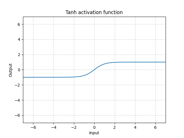
• torch.nn.Tanh()：对输入的每个元素，$f(x)=\frac{e^x-e^{-x}}{e^x+e^{-x}}$
  

import torch
from torch import nn
m = nn.Tanh()
input = torch.randn(6)
print(input)
# tensor([-1.4601, -0.1697,  0.7304, -0.7290,  1.1595,  0.0045])
print(m(input))
# tensor([-0.8977, -0.1681,  0.6233, -0.6225,  0.8209,  0.0045])

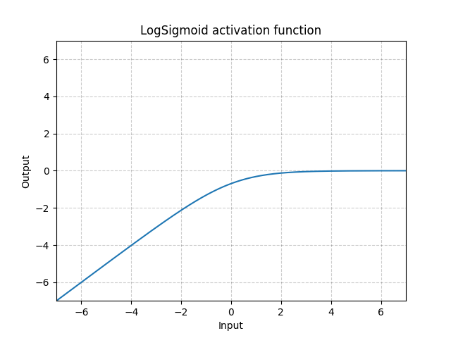
• torch.nn.LogSigmoid()：对输入的每个元素， $LogSigmoid(x)=log(1/(1+e^{-x}))$
  

import torch
from torch import nn
m = nn.LogSigmoid()
input = torch.randn(6)
print(input)
# tensor([-1.2238, -0.1355, -0.4778,  0.9836, -0.3558,  2.2939])
print(m(input))
# tensor([-1.4817, -0.7632, -0.9603, -0.3177, -0.8868, -0.0961])

• torch.nn.Softplus(beta=1, threshold=20)：对每个元素运用 Softplus 函数， Softplus 定义如下：$f(x)=\frac{1}{\beta }\ast log(1+e^{\beta \ast x})$
  Softplus 函数是 ReLU 函数的平滑逼近， Softplus 函数可以使得输出值限定为正数。
  为了保证数值稳定性，线性函数的转换可以使输出大于某个值。
  
  参数：
  （1）beta： Softplus 函数的 beta 值
  （2） threshold：阈值

import torch
from torch import nn
m = nn.Softplus()
input = torch.randn(6)
print(input)
# tensor([ 0.3301,  1.3399, -0.6725, -1.7277,  0.1790,  1.7915])
print(m(input))
# tensor([0.8717, 1.5725, 0.4124, 0.1636, 0.7866, 1.9457])

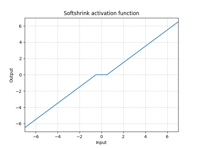
• torch.nn.Softshrink(lambd=0.5)：对每个元素运用 Softshrink 函数， Softshrink 函数定义如下：
  $$SoftShrinkage(x)=\{\begin{array}{ll}x-\lambda & x>\lambda \\ x+\lambda & x<-\lambda \\ 0& otherwise\end{array}$$
  

import torch
from torch import nn
m = nn.Softshrink()
input = torch.randn(6)
print(input)
# tensor([-0.1473, -1.0722,  2.3532, -0.6775,  0.1545,  0.1195])
print(m(input))
# tensor([ 0.0000, -0.5722,  1.8532, -0.1775,  0.0000,  0.0000])

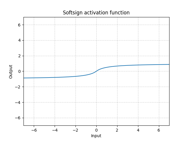
• torch.nn.Softsign()：逐元素使用以下操作：$SoftSign(x)=\frac{x}{1+|x|}$
  

import torch
from torch import nn
m = nn.Softsign()
input = torch.randn(6)
print(input)
# tensor([-1.1256,  0.6065, -1.7092,  0.5611,  0.7284,  1.5538])
print(m(input))
# tensor([-0.5295,  0.3775, -0.6309,  0.3594,  0.4214,  0.6084])

• torch.nn.Softmin(dim=None)：对 n 维输入张量运用 Softmin 函数，将张量的每个元素缩放到（0,1）区间且和为 1。
  $Softmin(x_i)=\frac{e^{-x_i}}{{\sum }_j{e}^{-x_j}}$

import torch
from torch import nn
m = nn.Softmin()
input = torch.randn(2, 3)
print(input)
# tensor([[-0.9406, -0.7574, -0.2140],[ 1.0005, -1.2016,  0.1894]])
print(m(input))
# tensor([[0.4318, 0.3595, 0.2088],[0.0813, 0.7356, 0.1830]])

• torch.nn.Softmax(dim=None)：对 输入张量的dim维度运用 Softmax 函数，将张量的dim维度每个元素缩放到（ 0,1）区间且和为 1。 Softmax 函数定义如下：$Softmax(x_i)=\frac{e^{x_i}}{{\sum }_j{e}^{x_j}}$

import torch
from torch import nn
m = nn.Softmax()
input = torch.randn(2, 3)
print(input)
# tensor([[ 1.1853, -0.9699, -0.6635], [ 0.2013,  0.8596, -2.3155]])
print(m(input))
# tensor([[0.7854, 0.0910, 0.1236],[0.3320, 0.6412, 0.0268]])

• torch.nn.LogSoftmax(dim=None)：对 输入张量的dim维度运用 LogSoftmax函数，函数定义如下：$LogSoftmax(x_i)=log(\frac{e^{x_i}}{{\sum }_j{e}^{x_j}})$

import torch
from torch import nn
m = nn.LogSoftmax()
input = torch.randn(2, 3)
print(input)
# tensor([[ 0.3179, -1.6143, -0.0478],[ 0.7923, -1.6657, -2.5130]])
print(m(input))
# tensor([[-0.6090, -2.5411, -0.9746],[-0.1154, -2.5733, -3.4206]])

2.归一化层

• torch.nn.BatchNorm1d(num_features, eps=1e-05, momentum=0.1, affine=True, track_running_stats=True, device=None, dtype=None)：
  输入尺寸：$(N,C)or(N,C,L)$
  输出尺寸：$(N,C)or(N,C,L)$ (与输入尺寸相同)
  在训练时，该层计算每次输入的均值与方差，并进行移动平均。移动平均默认的动量值为 0.1。
  在验证时，训练求得的均值/方差将用于标准化验证数据。
  重要参数：
  （1）momentum： 动态均值和动态方差所使用的动量。默认为 0.1。
  （2）affine： 一个布尔值，当设为 true，给该层添加可学习的仿射变换参数

import torch
from torch import nn
m1 = nn.BatchNorm1d(5)  # 默认有可学习参数
m2 = nn.BatchNorm1d(5,affine=False)  # 没有可学习参数
input = torch.randn(2, 5)
print(input)
# tensor([[-0.1493,  0.6807,  0.2940,  1.6287, -0.9222],
#         [-1.7403, -0.7764, -0.6606, -0.2361, -0.1404]])
print(m1(input))
# tensor([[ 1.0000,  1.0000,  1.0000,  1.0000, -1.0000],
#         [-1.0000, -1.0000, -1.0000, -1.0000,  1.0000]],
#        grad_fn=<NativeBatchNormBackward>)
print(m2(input))
# tensor([[ 1.0000,  1.0000,  1.0000,  1.0000, -1.0000],
#         [-1.0000, -1.0000, -1.0000, -1.0000,  1.0000]])

• torch.nn.BatchNorm2d(num_features, eps=1e-05, momentum=0.1, affine=True, track_running_stats=True, device=None, dtype=None)：对小批量(mini-batch)3d 数据组成的 4d 输入进行批标准化(Batch Normalization)操作
  输入尺寸：$(N,C,H,W)$
  输出尺寸：$(N,C,H,W)$ (与输入尺寸相同)
  在训练时，该层计算每次输入的均值与方差，并进行移动平均。移动平均默认的动量值为 0.1。
  在验证时，训练求得的均值/方差将用于标准化验证数据。
  重要参数：
  （1）momentum： 动态均值和动态方差所使用的动量。默认为 0.1。
  （2）affine： 一个布尔值，当设为 true，给该层添加可学习的仿射变换参数
  输入：（ N, C, H, W) - 输出：（ N, C, H, W）（输入输出相同）

import torch
from torch import nn
m1 = nn.BatchNorm2d(5)  # 默认有可学习参数
m2 = nn.BatchNorm2d(5,affine=False)  # 没有可学习参数
input = torch.randn(2, 5, 35, 45)
print(m1(input).shape)
# torch.Size([2, 5, 35, 45])
print(m2(input).shape)
# torch.Size([2, 5, 35, 45])

• torch.nn.BatchNorm3d(num_features, eps=1e-05, momentum=0.1, affine=True)：对小批量(mini-batch)4d 数据组成的 5d 输入进行批标准化(Batch Normalization)操作
  参数：
  （1）num_features： 来自期望输入的特征，该期望输入的大小 (N, C, D, H, W)
  （2）eps： 为保证数值稳定性（分母不能趋近或取 0） ,给分母加上的值。默认为 1e-5。
  （3）momentum： 动态均值和动态方差所使用的动量。默认为 0.1。
  （4）affine： 一个布尔值，当设为 true，给该层添加可学习的仿射变换参数。即$\alpha 与\gamma$
  输入：（ N, C, D, H, W) - 输出：（ N, C, D, H, W）（输入输出相同）

import torch
from torch import nn
m1 = nn.BatchNorm3d(3)  # 默认有可学习参数
m2 = nn.BatchNorm3d(3,affine=False)  # 没有可学习参数
input = torch.randn(2, 3, 35, 45, 10)
print(m1(input).shape)
# torch.Size([2, 3, 35, 45, 10])
print(m2(input).shape)
# torch.Size([2, 3, 35, 45, 10])

3.线性层

• torch.nn.Linear(in_features, out_features, bias=True)：对输入数据做线性变换： y=Ax+b
  参数：
  （1）in_features - 每个输入样本的大小
  （2）out_features - 每个输出样本的大小
  （3）bias - 若设置为 False，这层不会学习偏置。默认值： True
  输入大小：(N,in_features)
  输出大小：(N,out_features)

import torch
from torch import nn
m = nn.Linear(20, 30)
input = torch.randn(12, 20)
print(m(input).shape)
# torch.Size([12, 30])

4.Dropout 层

• torch.nn.Dropout(p=0.5, inplace=False)：随机将输入张量中部分元素设置为 0。对于每次前向调用，被置 0 的元素都是随机的。
  参数：
  （1）p - 将元素置 0 的概率。默认值： 0.5
  （2）in-place - 若设置为 True，会在原地执行操作。默认值： False
  形状：
  （1）输入： 任意。输入可以为任意形状。
  （2）输出： 输出和输入形状相同。

import torch
from torch import nn
m = nn.Dropout(p=0.2)
input = torch.randn(20, 16)
print(m(input).shape)
# torch.Size([20, 16])

• torch.nn.Dropout2d(p=0.5, inplace=False)：随机将输入张量中整个通道设置为 0。对于每次前向调用，被置 0 的通道都是随机的，通常输入来自 Conv2d 模块。
  参数：
  （1）p - 将元素置 0 的概率。默认值： 0.5
  （2）in-place - 若设置为 True，会在原地执行操作。默认值： False
  形状：
  （1） 输入： (N,C,H,W)
  （2） 输出： (N,C,H,W)（与输入形状相同）

import torch
from torch import nn
m = nn.Dropout2d(p=0.2)
input = torch.randn(20, 16, 32, 32)
print(m(input).shape)
# torch.Size([20, 16, 32, 32])

torch.nn.Dropout3d(p=0.5, inplace=False)：随机将输入张量中整个通道设置为 0。对于每次前向调用，被置 0 的通道都是随机的，通常输入来自 Conv3d 模块。
参数：
（1）p - 将元素置 0 的概率。默认值： 0.5
（2）in-place - 若设置为 True，会在原地执行操作。默认值： False
形状：
（1） 输入： (N,C,D,H,W)
（2） 输出： (N,C,D,H,W)（与输入形状相同）

import torch
from torch import nn
m = nn.Dropout3d(p=0.2)
input = torch.randn(20, 16, 4, 32, 32)
print(m(input).shape)
# torch.Size([20, 16, 4, 32, 32])

5.距离函数

• torch.nn.PairwiseDistance(p=2, eps=1e-06)：按批计算向量 v1, v2 之间的距离
  参数：
  （1）x (Tensor): 包含两个输入 batch 的张量
  （2）p (real): 范数次数，默认值： 2
  形状：
  （1）输入： (N,D)，其中 D=向量维数
  （2）输出： (N,1)

import torch
from torch import nn
pdist = nn.PairwiseDistance(2)
input1 = torch.arange(12).reshape(3,4)
input2 = torch.arange(12).reshape(3,4)
print(input1, input2)
output = pdist(input1, input2)
print(output)
# tensor([2.0000e-06, 2.0000e-06, 2.0000e-06])

6.损失函数

基本用法：
criterion = LossCriterion() #构造函数有自己的参数
loss = criterion(x, y) #调用标准时也有参数
计算出来的结果已经对 mini-batch 取了平均。

• torch.nn.L1Loss(size_average=None, reduce=None, reduction='mean')：创建一个衡量输入 x(模型预测输出)和目标 y 之间差的绝对值的平均值的标准。
  $$loss(x,y)=\frac{1}{n}\sum |x_i-y_i|$$
  形状：
  x尺寸：(N,∗) ，*表示任意值
  y尺寸：同上
  输出尺寸：标量，如果reduction=none，那么输出尺寸与输入的x或y尺寸相同
  如果在创建 L1Loss 实例的时候在构造函数中传入 size_average=False，那么求出来的绝对值的和将不会除以 n。

import torch
from torch import nn
loss = nn.L1Loss()
input = torch.randn(3, 5)
target = torch.randn(3, 5)
output = loss(input, target)
print(output)
# tensor(1.1191)

loss = nn.L1Loss(reduction="none")
output = loss(input, target)
print(output)
# tensor([[2.6041, 0.7351, 3.2098, 0.6427, 1.4476],
#         [1.3020, 0.0344, 1.3406, 0.4832, 0.7455],
#         [0.4987, 0.1257, 0.3320, 2.7098, 0.5757]])
print(output.sum())
# tensor(16.7869)
print(output.mean())
# tensor(1.1191)

• torch.nn.MSELoss(size_average=True)：创建一个衡量输入 x(模型预测输出)和目标 y 之间均方误差标准。
  $$loss(x,y)=\frac{1}{n}\sum (x_i-y_i{)}^2$$
  形状：
  x尺寸：(N,∗) ，*表示任意值
  y尺寸：同上
  输出尺寸：标量，如果reduction=none，那么输出尺寸与输入的x或y尺寸相同
  如果在创建 L2Loss 实例的时候在构造函数中传入 size_average=False，那么求出来的绝对值的和将不会除以 n。

import torch
from torch import nn
loss = nn.MSELoss()
input = torch.randn(3, 5)
target = torch.randn(3, 5)
output = loss(input, target)
print(output)
# tensor(2.8648)

loss = nn.MSELoss(reduction="none")
output = loss(input, target)
print(output)
# tensor([[3.1276e-01, 1.6991e+00, 2.4922e-03, 1.1089e-01, 3.8143e-01],
#         [5.8569e-01, 1.1830e+00, 1.4926e+00, 7.7746e+00, 9.6769e-04],
#         [8.2330e+00, 2.9971e+00, 5.6262e+00, 4.6929e-01, 1.2102e+01]])
print(output.sum())
# tensor(42.9715)
print(output.mean())
# tensor(2.8648)

• torch.nn.CrossEntropyLoss(weight=None, size_average=True)：此标准将 LogSoftMax 和 NLLLoss 集成到一个类中，当训练一个多类分类器的时候，这个方法是十分有用的。
  （1）weight(tensor): 1D tensor， n 个元素，分别代表 n 类的权重，如果你的训练样本很不均衡的话，是非常有用的。默认值为 None。
  （2）input : 包含每个类的得分， 2D tensor,shape 为 batch*n
  （3）target: 大小为 n 的 1D tensor，包含类别的索引(0 到 n-1)。

import torch
from torch import nn
loss = nn.CrossEntropyLoss()
input = torch.randn(3, 5)
target = torch.empty(3, dtype=torch.long).random_(5)
print(target.shape)
# torch.Size([3])
output = loss(input, target)
print(output)
# tensor(2.3181)

• torch.nn.NLLLoss(weight=None, size_average=True)：负的 log likelihood loss 损失。用于训练一个 n 类分类器。
  如果提供weight 参数的话， weight 参数应该是一个 1D tensor，里面的值对应类别的权重。当你的训练集样本不均衡的话，使用这个参数是非常有用的。
  输入是一个包含类别 log-probabilities 的 2-D tensor，形状是(mini-batch， n)可以通过在最后一层加 LogSoftmax 来获得类别的 log-probabilities。
  如果您不想增加一个额外层的话，您可以使用 CrossEntropyLoss。
  此 loss 期望的 target 是类别的索引 (0 to N-1, where N = number of classes)
  参数说明：
  （1）weight (Tensor, optional) – 手动指定每个类别的权重。如果给定的话，必须是长度为 nclasses
  （2） size_average (bool, optional) – 默认情况下，会计算 mini-batch``loss 的平均值。然而，如果size_average=False 那么将会把 mini-batch 中所有样本的 loss 累加起来。
  形状:
  （1）Input: (N,C) , C 是类别的个数
  （2）Target: (N) ， target 中每个值的大小满足 0 <= targets[i] <= C-1

import torch
from torch import nn
m = nn.LogSoftmax(dim=-1)
loss = nn.NLLLoss()
input = torch.randn(3, 5)
target = torch.LongTensor([1, 0, 4])
output = loss(m(input), target)
print(output)
# tensor(2.5302)

• torch.nn.NLLLoss2d(weight=None, size_average=True)：对于图片的 negative log likehood loss。计算每个像素的 NLL loss。现在已经被废弃，集成到NLLLoss里面了
  参数说明：
  （1）weight (Tensor, optional) – 用来作为每类的权重，如果提供的话，必须为 1-Dtensor，大小为 C：类别的个数。
  （2）size_average – 默认情况下，会计算 mini-batch loss 均值。如果设置为 False 的话，将会累加 mini-batch中所有样本的 loss 值。默认值： True。
  形状：
  （1）Input: (N,C,H,W) C 类的数量
  （2）Target: (N,H,W) where each value is 0 <= targets[i] <= C-1

import torch
from torch import nn
conv = nn.Conv2d(16, 32, (3, 3)).float()  # 此处的32就是类别数
m = nn.LogSoftmax(dim=1)  # 首先要使用LogSoftmax
loss = nn.NLLLoss2d()  # 再使用NLLLoss
loss2 = nn.NLLLoss()
input = torch.randn(3, 16, 10, 10)
target = torch.LongTensor(3, 8, 8).random_(0, 4)  # each element in target has to have 0 <= value < Classes
print(target.shape)
# torch.Size([3, 8, 8])
convOut = conv(input)
print(m(convOut).shape)
# torch.Size([3, 32, 8, 8])  #  (Batch,Classes,height,width)
output = loss(m(convOut) , target)
print(output)
# tensor(3.6891, grad_fn=<NllLoss2DBackward>)
output = loss2(m(convOut) , target)
print(output)
# tensor(3.6891, grad_fn=<NllLoss2DBackward>)

• torch.nn.KLDivLoss(weight=None, size_average=True)：计算 KL 散度损失，KL 散度常用来描述两个分布的距离。与 NLLLoss 一样，给定的输入应该是 log-probabilities。然而。和 NLLLoss 不同的是， input 不限于2-D tensor，因为此标准是基于 element 的。target 应该和 input 的形状相同。默认情况下， loss 会基于 element 求平均。如果 size_average=False loss 会被累加起来。

import torch
from torch import nn
conv = nn.Conv2d(16, 32, (3, 3)).float()  # 此处的32就是类别数
m = nn.LogSoftmax(dim=1)  # 首先要使用LogSoftmax
loss= nn.KLDivLoss()
input = torch.randn(3, 16, 10, 10)
target = torch.Tensor(3, 32, 8, 8).random_(0, 4)  # each element in target has to have 0 <= value < Classes
print(target.shape)
# torch.Size([3, 32, 8, 8])
convOut = conv(input)
print(m(convOut).shape)
# torch.Size([3, 32, 8, 8])  #  (Batch,Classes,height,width)
output = loss(m(convOut) , target)
print(output)
# tensor(6.6287, grad_fn=<KlDivBackward>)

• torch.nn.BCELoss(weight=None, size_average=True)：计 算 target 与 output 之 间 的 二值交叉熵。
  $$loss(o,t)=-\frac{1}{n}\sum _i(t[i]log(o[i])+(1-t[i])log(1-o[i]))$$ 如 果 weight 被 指 定 ：
  $$loss(o,t)=-\frac{1}{n}\sum _{i}weights[i](t[i]log(o[i])+(1-t[i])\ast log(1-o[i]))$$
  注意 0<=t[i]<=1。
  默认情况下， loss 会基于 element 平均，如果 size_average=False 的话， loss 会被累加。
  形状
  （1）input：(∗)，其中* 表示任何数量的尺寸。
  （2）target：与输入尺寸相同
  （3）output：标量，如果reduction = 'none'，则与输入尺寸相同

import torch
from torch import nn
m = nn.Sigmoid()
loss = nn.BCELoss()
input = torch.randn(2, 3, requires_grad=True)
target = torch.empty(2, 3).random_(2)
output = loss(m(input), target)
print(output)
# tensor(0.7017, grad_fn=<BinaryCrossEntropyBackward>)

• torch.nn.SmoothL1Loss(size_average=True)：平滑版本L1 loss。
  $$l_n=\{\begin{array}{ll}\frac{1}{2\beta }(x_n-y_n{)}^2& |x_n-y_n|<\beta \\ |x_n-y_n|-\frac{1}{2\beta }& otherwise\end{array}$$
  形状
  （1）input：(∗)，其中* 表示任何数量的尺寸。
  （2）target：与输入尺寸相同
  （3）output：标量，如果reduction = 'none'，则与输入尺寸相同

import torch
from torch import nn
loss = nn.SmoothL1Loss()
input = torch.randn(3, 1)
target = torch.randn(3, 1)
output = loss(input, target)
print(output)
# tensor(0.6970)

• torch.nn.BCEWithLogitsLoss(weight=None, size_average=True)：计 算 target 与 output 之 间 的 二值交叉熵，将Sigmoid层和BCELoss合并在一个类中。
  $$loss(o,t)=-\frac{1}{n}\sum _i(t[i]log(o[i])+(1-t[i])log(1-o[i]))$$ 如 果 weight 被 指 定 ：
  $$loss(o,t)=-\frac{1}{n}\sum _{i}weights[i](t[i]log(o[i])+(1-t[i])\ast log(1-o[i]))$$
  注意 0<=t[i]<=1。
  默认情况下， loss 会基于 element 平均，如果 size_average=False 的话， loss 会被累加。
  形状
  （1）input：(∗)，其中* 表示任何数量的尺寸。
  （2）target：与输入尺寸相同
  （3）output：标量，如果reduction = 'none'，则与输入尺寸相同

import torch
from torch import nn
loss = nn.BCEWithLogitsLoss()
input = torch.randn(2, 3, requires_grad=True)
target = torch.empty(2, 3).random_(2)
output = loss(input, target)
print(output)
# tensor(0.8615, grad_fn=<BinaryCrossEntropyWithLogitsBackward>)

参考目录

https://blog.csdn.net/weixin_40920183/article/details/119814472