深度学习05 - 一阶全卷积目标检测实例（FCOS）

一阶全卷积目标检测实例：

Fully-Convolutional One-Stage Object Detection

参考：EECS 498-007/598-005 Assignment 4-1: One-Stage Object Detector

论文地址：

 FCOS: Fully Convolutional One-Stage Object Detection

FCOS: A Simple and Strong Anchor-free Object Detector

FCOS概述：

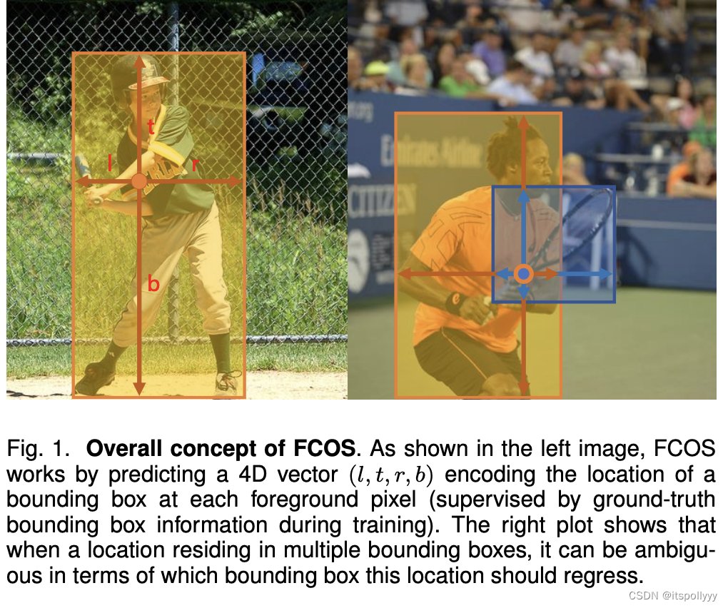
不同于使用Anchor去确定目标，FCOS是使用全卷积网络通过确定特征图上的每个位置来预测该点距离目标的距离（左上右下 LTRB），如下图：

FCOS: A Simple and Strong Anchor-free Object Detector

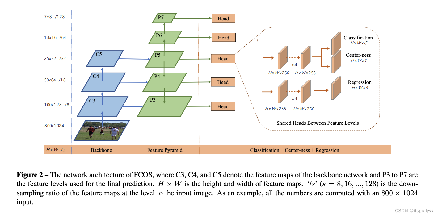
流程：

该流程与第一版的网络的不同点在于最后将regression 和centre-ness分支放在一起。该文中使用的是第二版的网络。

FCOS: Fully Convolutional One-Stage Object Detection​​​​​​

FCOS: A Simple and Strong Anchor-free Object Detector

​

1. 实现backbone 和 Feature Pyramid 网络 

1. Backbone：

用RegNetX-400MF网络作为backbone

​

在backbone中，使用RegNetX-400MF作为网络，在卷积层后输出特征C3，C4，C5。得到特征C3，C4，C5后通过1x1的卷积层得到减少通道尺寸后的特征，然后从上往下进行融合。在融合的时候，因为特征的大小不一样，所以将上一个特征进行两倍的上采样，通过Nearest Neighbor上采样。再将每层的特征再进行3x3，pooling为1的卷积得到新的特征图。

其中1x1的卷积的实现：

题目中要求输出相同

# Add THREE lateral 1x1 conv and THREE output 3x3 conv layers.
self.fpn_params = nn.ModuleDict()
# Replace "pass" statement with your code

self.fpn_params['l3'] = nn.Conv2d(dummy_out_shapes[0][1][1], self.out_channels, 1, 1, 0)
self.fpn_params['l4'] = nn.Conv2d(dummy_out_shapes[1][1][1], self.out_channels, 1, 1, 0)
self.fpn_params['l5'] = nn.Conv2d(dummy_out_shapes[2][1][1], self.out_channels, 1, 1, 0)

lat3 = self.fpn_params['l3'](backbone_feats['c3'])  # [2, 64, 28, 28]
lat4 = self.fpn_params['l4'](backbone_feats['c4'])  # [2, 64, 14, 14]
lat5 = self.fpn_params['l5'](backbone_feats['c5'])  # [2, 64, 7, 7]

ModuleDict类：

用字典存放卷积层和网络

Holds submodules in a dictionary.

ModuleDict can be indexed like a regular Python dictionary, but modules it contains are properly registered, and will be visible by all Module methods.

ModuleDict is an ordered dictionary that respects

• the order of insertion, and

• in update(), the order of the merged OrderedDict, dict (started from Python 3.6) or another ModuleDict (the argument to update()).

Note that update() with other unordered mapping types (e.g., Python’s plain dict before Python version 3.6) does not preserve the order of the merged mapping.

Parameters

modules (iterable, optional) – a mapping (dictionary) of (string: module) or an iterable of key-value pairs of type (string, module)

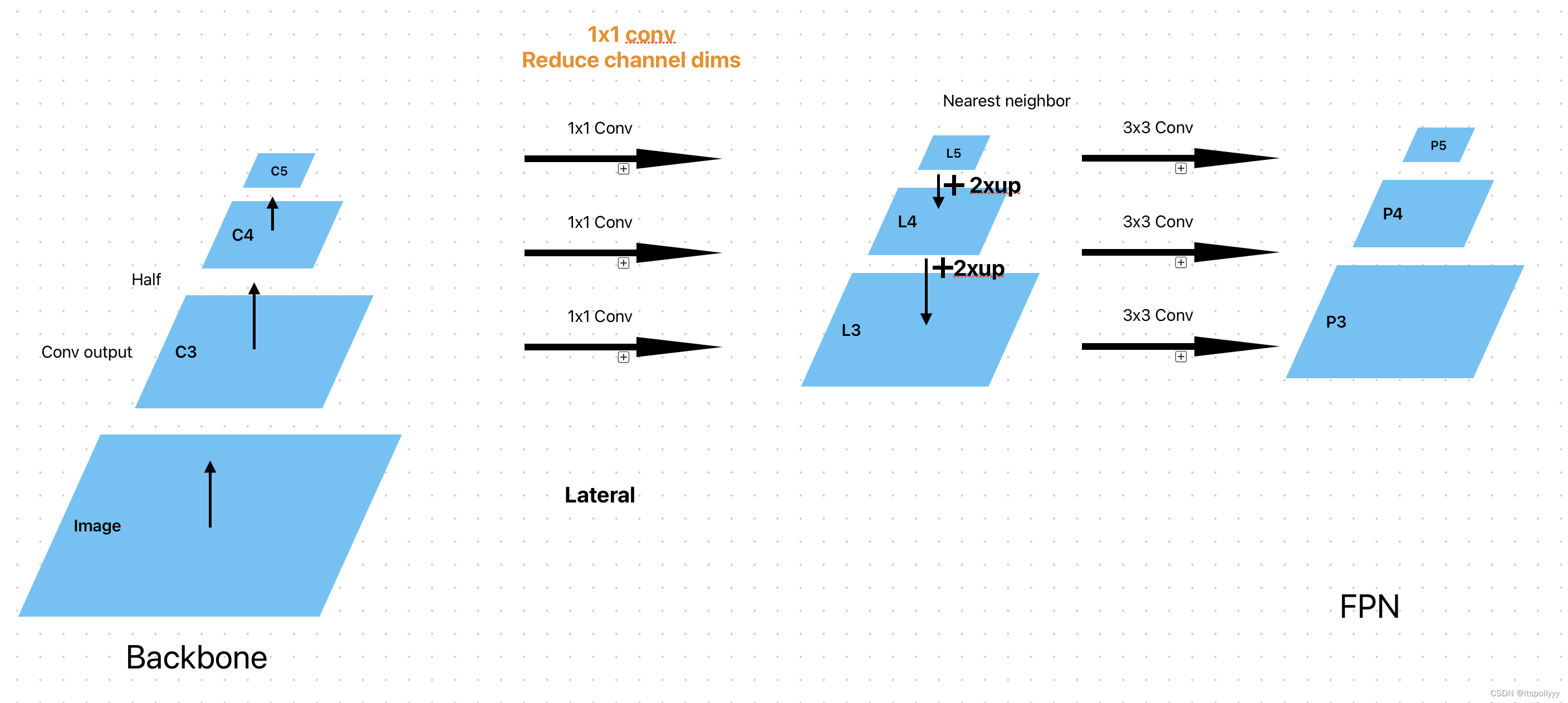
2.FPN网络

关于FPN网络，论文中的解释如图：

Feature Pyramid Networks for Object Detection

输入的图像通过卷积后，得到C3，C4，C5特征图，然后将特征图进行一个1x1的卷积，得到新的特征图，将新的特征图用2倍的缩放，使用nearest neighbor上采样。将上层的特征图与下层的特征图进行融合。

关于为什么是2倍：因为在图像进行卷积的时候，stide是8，16，32每次都是上一次的2倍。

通过使用F.interpolate将l5和l4的大小放大到跟l4和l3一样。

lat5_resize = nn.functional.interpolate(lat5, size=(lat4.shape[2], lat4.shape[3]), mode='nearest')  # (14, 14)
# merge after convolution lat4 with lat5_resize (2x upsample)
lat4 = lat4 + lat5_resize
lat4_resize = nn.functional.interpolate(lat4, size=(lat3.shape[2], lat3.shape[3]), mode='nearest')
# merge lat4_resize with lat3
lat3 = lat3 + lat4_resize

将新的特征图，再进行3x3的卷积，其中padding是1，stride是1。得到proposal 特征图P3，P4，P5。

self.fpn_params['p3'] = nn.Conv2d(self.out_channels, self.out_channels, 3, 1, 1)
self.fpn_params['p4'] = nn.Conv2d(self.out_channels, self.out_channels, 3, 1, 1)
self.fpn_params['p5'] = nn.Conv2d(self.out_channels, self.out_channels, 3, 1, 1)

fpn_feats['p3'] = self.fpn_params['p3'](lat3)
fpn_feats['p4'] = self.fpn_params['p4'](lat4)
fpn_feats['p5'] = self.fpn_params['p5'](lat5)

视频1.1.2 FPN结构详解也提供了更详细的结构可供参考。

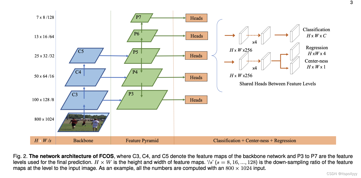
2.实现预测网络（Head）

通过实现Head来预测分类，bounding box和center-ness

在预测网络中，拿到前项输出的特征图后，喂给卷积层。

拿classification这一分支来讲，特征图输入给3x3的卷积层然后在给激活函数ReLU，然后再输入给相同的3x3的卷积层+ReLU，最后再进行一次3x3的卷积，得到classification。此时classification的shape跟输入的特征图的shape不一样。输入特征图的shape为(B, C, H, W)， 而classification的shape为(B, H*W, C)。同理centre-ness和bounding box的shape为(B, H*W, 1)和(B, H*W, 4) 此处的4 是bounding box的四个点。

1. 搭建3x3的卷积层，其中权重的均值为0，标准差为0.01， 偏差为0

循环的使用将输出两层卷积层

对应图中这部分

inputSize = in_channels
for out_channel in stem_channels:
    print('out_channel', out_channel)
    # class
    conv1 = nn.Conv2d(inputSize, out_channel, 3, 1, 1)
    relu1 = nn.ReLU()
    # init weight
    torch.nn.init.normal_(conv1.weight, 0, 0.01)
    # init bias
    # torch.nn.init.constant_(conv1.bias, 0)
    torch.nn.init.zeros_(conv1.bias)
    # append conv1 and relu1 to stem_cls
    stem_cls.append(conv1)
    stem_cls.append(relu1)

    # box
    conv2 = nn.Conv2d(inputSize, out_channel, 3, 1, 1)
    relu2 = nn.ReLU()
    # init weight
    torch.nn.init.normal_(conv2.weight, 0, 0.01)
    # init bias
    # torch.nn.init.constant_(conv1.bias, 0)
    torch.nn.init.zeros_(conv2.bias)
    # append conv1 and relu1 to stem_cls
    stem_box.append(conv2)
    stem_box.append(relu2)
    inputSize = out_channel

2. 为三个不同的预测值搭建一个3x3的卷积层

self.pred_cls = nn.Conv2d(stem_channels[-1], num_classes, 3, 1, 1)
torch.nn.init.normal_(self.pred_cls.weight, 0, 0.01)
torch.nn.init.zeros_(self.pred_cls.bias)

self.pred_box = nn.Conv2d(stem_channels[-1], 4, 3, 1, 1)
torch.nn.init.normal_(self.pred_box.weight, 0, 0.01)
torch.nn.init.zeros_(self.pred_box.bias)

self.pred_ctr = nn.Conv2d(stem_channels[-1], 1, 3, 1, 1)
torch.nn.init.normal_(self.pred_ctr.weight, 0, 0.01)
torch.nn.init.zeros_(self.pred_ctr.bias)

3. forward

组装一下之前的卷积层，得到三个预测值

feats_per_fpn_level 是前面FPN网络传递过来的特征{p3,p4,p5},每个特征的shape是(batch_size, fpn_channels, H, W)。最终我们要得到这三个预测值的shape分别为：
        1. Classification logits: `(batch_size, H * W, num_classes)`.
        2. Box regression deltas: `(batch_size, H * W, 4)`
        3. Centerness logits:     `(batch_size, H * W, 1)`

流程：特征->stem 层-> pred层；

（⚠️：需reshape到目标值的shape，使用view()和permute()）

for level, feature in feats_per_fpn_level.items():

    # append each level's feature into dict
    class_logits[level] = self.pred_cls(self.stem_cls(feature))
    # print('========1', class_logits[level].shape)   # ([2, 20, 14, 14])
    # reshape Classification logits: `(batch_size, H * W, num_classes)`.
    batch_size = class_logits[level].shape[0]
    num_cls = class_logits[level].shape[1]
    # reshape [2, 20, 14, 14] to [2, 14*14, 20]
    # -1 => 2*20*14*14/2*20
    # permute into desire order
    class_logits[level] = class_logits[level].view(batch_size, num_cls, -1).permute(0, 2, 1)

    boxreg_deltas[level] = self.pred_box(self.stem_box(feature))
    # reshape Box regression deltas: `(batch_size, H * W, 4)`
    boxreg_deltas[level] = boxreg_deltas[level].view(batch_size, 4, -1).permute(0, 2, 1)

    centerness_logits[level] = self.pred_ctr(self.stem_box(feature))
    # reshape Centerness logits:     `(batch_size, H * W, 1)`
    centerness_logits[level] = centerness_logits[level].view(batch_size, 1, -1).permute(0, 2, 1)

3. 训练网络

前面讲到了整个网络的构成，此时来细剖整个网络是如何进行训练的。

不同于分类模型，输入的是照片和label，其中label一般都是one-hot 向量。但在该模型中，每张照片都有大量的预测框；每一类的标签不与整张照片相关联而是与预测框相关联。

在FCOS中，使用GT target（Ground Truth Target）。每个GT target关联了三个参数：类别，bounding box，centre-ness。因为最后输出的三个预测值都与FPN层输出的特征图的每个位置有关，所以我们可以将GT boxes直接与FPN层的特征图的位置相关联。而GT box由标签、左上角坐标及右下角坐标构成，是一个5维的向量。

1. 得到特征图中的每个位置

通过训练网络，我们首先要得到特征图中的每一个位置，有了位置我们才有预测框（bounding box），才能预测到目标。

resource

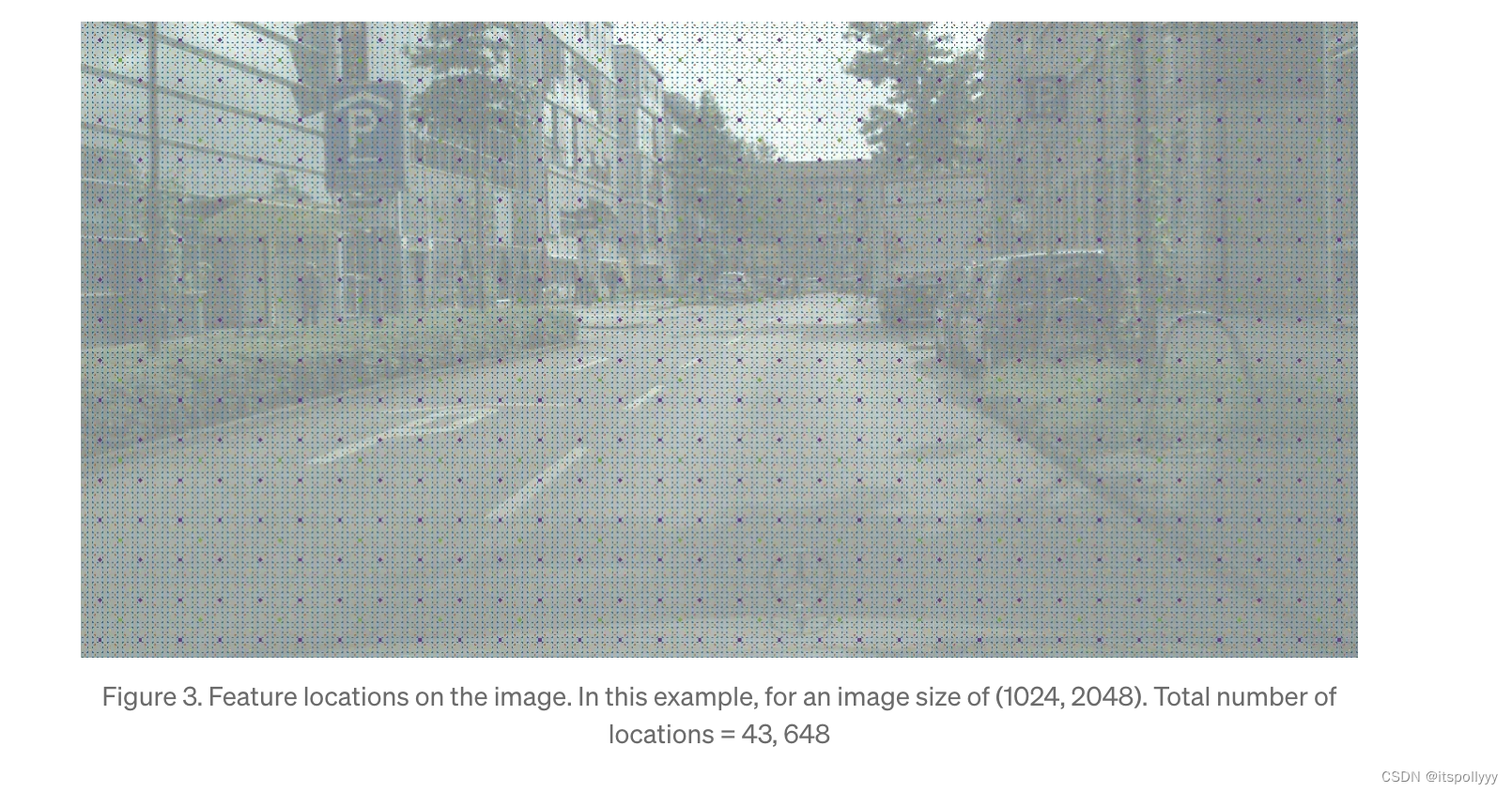
每层的特征图的大小为：(batch_size, channels, H / stride, W / stride)

特征图的位置：

1. i, j: 特征图的高和宽
2. 0.5：获取特征图中像素的中心
3. stride是在FPN网络中每层的stride:

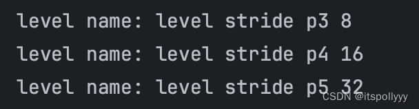
由此，我们可以通过循环FPN网络的每一层的特征图得到特征图的大小和stride，来计算位置。

# Replace "pass" statement with your code
# get x (0.5+i) i[0, 28(H)] ([2, 64, 28(H), 28(W)])
x = level_stride * torch.arange(0.5, feat_shape[2] + 0.5, step=1, device=device, dtype=dtype)
# get y (0.5+j) j [0, 28(W)] ([2, 64, 28(H), 28(W)])
y = level_stride * torch.arange(0.5, feat_shape[3] + 0.5, step=1, device=device, dtype=dtype)
# create a grid of these x y
(xGrid, yGrid) = torch.meshgrid(x, y, indexing='xy')
# xGrid shape [14, 14], [7, 7], [4, 4]
# add a new dimension of size 1 at the specified position (-1 in this case) in the tensor.
xGrid = xGrid.unsqueeze(dim=-1)
# print(xGrid.shape)
yGrid = yGrid.unsqueeze(dim=-1)
# concat these two and reshape to (H*W, 2)
location_coords[level_name] = torch.cat((xGrid,yGrid),dim=2).view(feat_shape[3]*feat_shape[2],2)
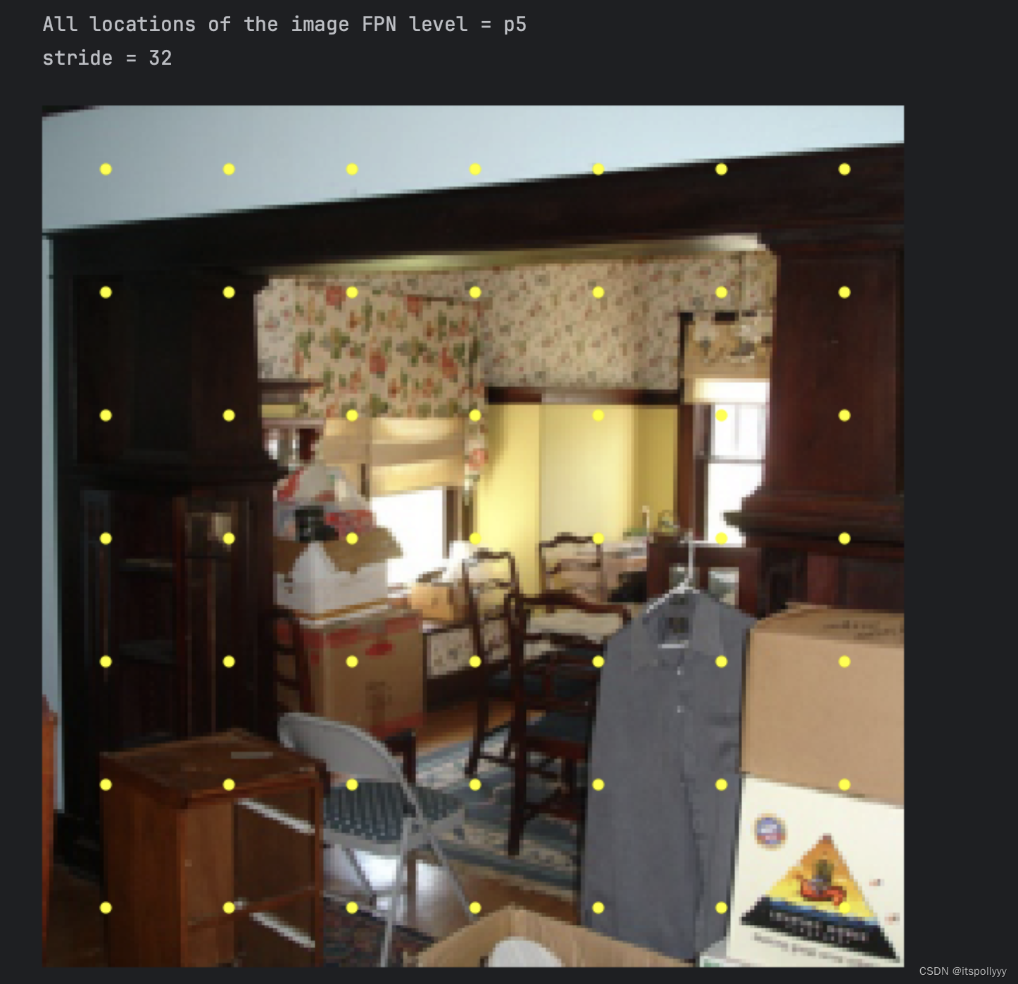
# print(torch.cat((xGrid, yGrid), dim=2).shape)

得到p3的位置图为

P4的位置图 

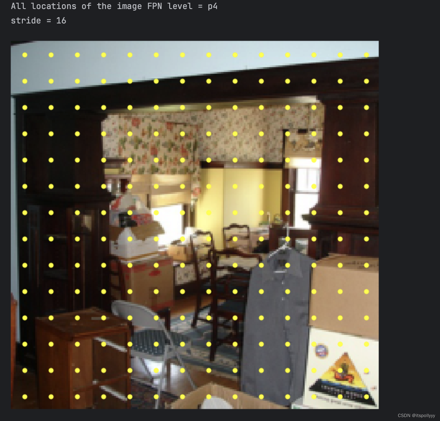
P5的位置图 

2. 将GT box和特征图的位置匹配

得到了特征图中的位置后，我们就可以与GT box相匹配了。

详细步骤参考论文中的3.2

def fcos_match_locations_to_gt(
    locations_per_fpn_level: TensorDict,
    strides_per_fpn_level: Dict[str, int],
    gt_boxes: torch.Tensor,
) -> TensorDict:
    """
    Match centers of the locations of FPN feature with a set of GT bounding
    boxes of the input image. Since our model makes predictions at every FPN
    feature map location, we must supervise it with an appropriate GT box.
    There are multiple GT boxes in image, so FCOS has a set of heuristics to
    assign centers with GT, which we implement here.

    NOTE: This function is NOT BATCHED. Call separately for GT box batches.

    Args:
        locations_per_fpn_level: Centers at different levels of FPN (p3, p4, p5),
            that are already projected to absolute co-ordinates in input image
            dimension. Dictionary of three keys: (p3, p4, p5) giving tensors of
            shape `(H * W, 2)` where H = W is the size of feature map.
        strides_per_fpn_level: Dictionary of same keys as above, each with an
            integer value giving the stride of corresponding FPN level.
            See `common.py` for more details.
        gt_boxes: GT boxes of a single image, a batch of `(M, 5)` boxes with
            absolute co-ordinates and class ID `(x1, y1, x2, y2, C)`. In this
            codebase, this tensor is directly served by the dataloader.

    Returns:
        Dict[str, torch.Tensor]
            Dictionary with same keys as `shape_per_fpn_level` and values as
            tensors of shape `(N, 5)` GT boxes, one for each center. They are
            one of M input boxes, or a dummy box called "background" that is
            `(-1, -1, -1, -1, -1)`. Background indicates that the center does
            not belong to any object.
    """

    matched_gt_boxes = {
        level_name: None for level_name in locations_per_fpn_level.keys()
    }

    # Do this matching individually per FPN level.
    for level_name, centers in locations_per_fpn_level.items():

        # Get stride for this FPN level.
        stride = strides_per_fpn_level[level_name]
        # get feature location's centre
        x, y = centers.unsqueeze(dim=2).unbind(dim=1)
        x0, y0, x1, y1 = gt_boxes[:, :4].unsqueeze(dim=0).unbind(dim=2)
        
        pairwise_dist = torch.stack([x - x0, y - y0, x1 - x, y1 - y], dim=2)

        # Pairwise distance between every feature center and GT box edges:
        # shape: (num_gt_boxes, num_centers_this_level, 4)
        pairwise_dist = pairwise_dist.permute(1, 0, 2)

        # The original FCOS anchor matching rule: anchor point must be inside GT.
        match_matrix = pairwise_dist.min(dim=2).values > 0

        # Multilevel anchor matching in FCOS: each anchor is only responsible
        # for certain scale range.
        # Decide upper and lower bounds of limiting targets.
        pairwise_dist = pairwise_dist.max(dim=2).values

        lower_bound = stride * 4 if level_name != "p3" else 0
        upper_bound = stride * 8 if level_name != "p5" else float("inf")
        match_matrix &= (pairwise_dist > lower_bound) & (
            pairwise_dist < upper_bound
        )

        # Match the GT box with minimum area, if there are multiple GT matches.
        gt_areas = (gt_boxes[:, 2] - gt_boxes[:, 0]) * (
            gt_boxes[:, 3] - gt_boxes[:, 1]
        )

        # Get matches and their labels using match quality matrix.
        match_matrix = match_matrix.to(torch.float32)
        match_matrix *= 1e8 - gt_areas[:, None]

        # Find matched ground-truth instance per anchor (un-matched = -1).
        match_quality, matched_idxs = match_matrix.max(dim=0)
        matched_idxs[match_quality < 1e-5] = -1

        # Anchors with label 0 are treated as background.
        matched_boxes_this_level = gt_boxes[matched_idxs.clip(min=0)]
        matched_boxes_this_level[matched_idxs < 0, :] = -1

        matched_gt_boxes[level_name] = matched_boxes_this_level

    return matched_gt_boxes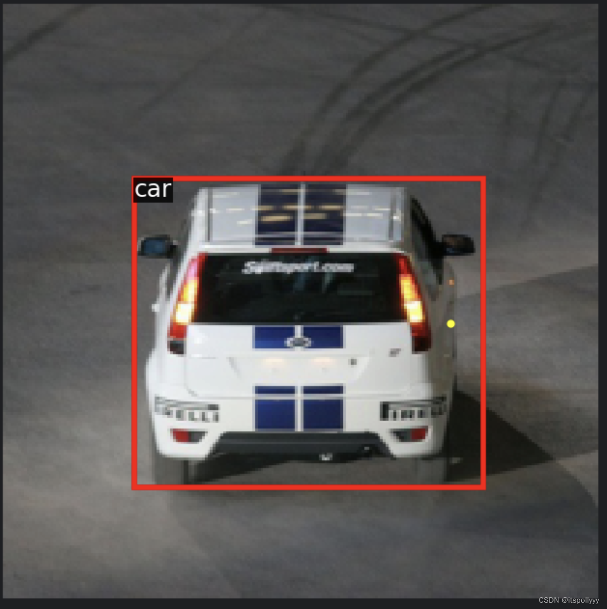

图中黄色的点是所选中的特征图的位置，

红色框是与之匹配的GT box

4. GT target 的候选框回归

候选框回归有四个预测值，分别是(left, top, right, bottom)，及特征图的位置到候选框的距离。

FCOS会用每层的stride来归一化这四个距离

在p3中， 

stride:8

位置（黄色点）：（xc， yc）shape(N, 2)

GT box：(x1, y1, x2, y2) shape(N, 4) 不含标签或(N, 5)含标签

l = (xc - x1) / stride              t = (yc - y1) / stride
r = (x2 - xc) / stride              b = (y2 - yc) / stride

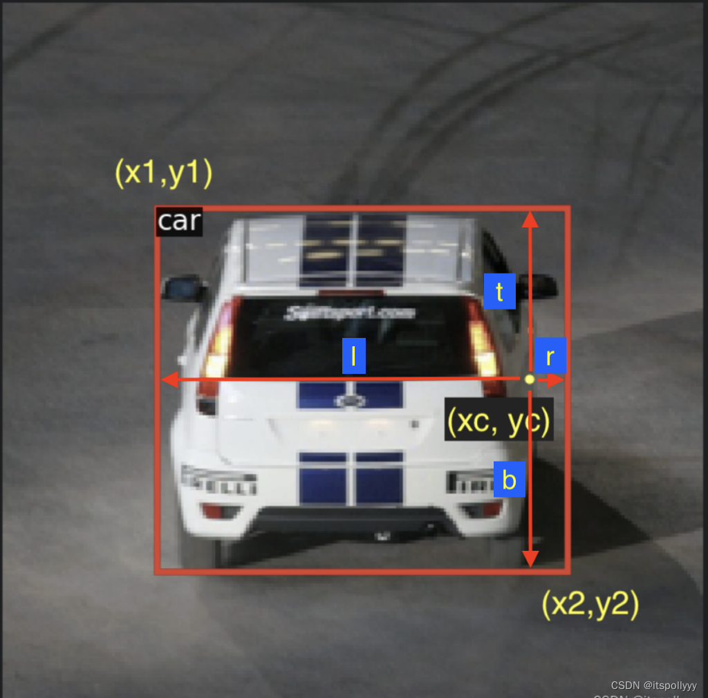
 用deltas来表示这四个距离的值，deltas的shape则为（N，4），参数4分别表示左（l），上（t），右（r），下（b）。

通过公式计算出LRTB的大小

deltas = torch.empty(gt_boxes.shape[0], 4).to(device=gt_boxes.device, dtype=gt_boxes.dtype)
# GT box have co-ordinates `(x1, y1, x2, y2)`
# location (xc, yc)
# l = (xc - x1) /stride
deltas[:, 0] = (locations[:, 0] - gt_boxes[:, 0]) / stride
#  t = (yc - y1) / stride
deltas[:, 1] = (locations[:, 1] - gt_boxes[:, 1]) / stride
#  r = (x2 - xc) / stride
deltas[:, 2] = (gt_boxes[:, 2] - locations[:, 0]) / stride
#  b = (y2 - yc) / stride
deltas[:, 3] = (gt_boxes[:, 3] - locations[:, 1]) / stride

如果GT box是背景的话，此时默认背景框的值为（-1，-1，-1，-1）或（-1，-1，-1，-1，-1），就要将deltas设置为（-1，-1，-1，-1）。

找到GT box中值为（-1，-1，-1，-1）的框。找到GT box的4四列，然后计算每行的和是否等于-4。若等于-4，那么置deltas为-1。

# If GT boxes are "background", then deltas must be `(-1, -1, -1, -1)`.
# You may assume that all the background boxes will be `(-1, -1, -1, -1)` or `(-1, -1, -1, -1, -1)`.
print('gt_boxes shape', gt_boxes.shape)
deltas[gt_boxes[:, :4].sum(dim=1) == -4] = -1

我们得到距离的值后，将其运用到特征图的位置上，得到目标边界框的坐标

link

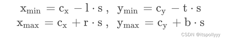
# x_min = c_x - l * s
# y_min = c_y - t * s
# x_max = c_x + r * s
# y_max = c_y + b * s
deltas = deltas.clip(min=0)
output_boxes = torch.empty(deltas.size()).to(device=deltas.device, dtype=deltas.dtype)

output_boxes[:, 3] = locations[:, 1] + stride * deltas[:, 3]
output_boxes[:, 2] = locations[:, 0] + stride * deltas[:, 2]
output_boxes[:, 1] = locations[:, 1] - stride * deltas[:, 1]
output_boxes[:, 0] = locations[:, 0] - stride * deltas[:, 0]

5.Centre-ness 

centre ness 是用来调整在模型中每个位置的分类的值。用于判断特征图上的某一像素距离检测框中心的距离。目的是为了提高模型的特征图的位置的准确度，第一版的论文也有指出为何centre ness 对模型特征图位置准确度提高有用。

centre-ness的计算公式如下：

 

center_ness = torch.empty(deltas.shape[0]).to(device=deltas.device, dtype=deltas.dtype)

center_ness = torch.sqrt(torch.min(deltas[:, 0], deltas[:, 2]) * torch.min(deltas[:, 1], deltas[:, 3]) /
                         torch.max(deltas[:, 0], deltas[:, 2]) * torch.max(deltas[:, 1], deltas[:, 3]))

6. loss

因为FCOS有三个预测值，分别对应三个不同的分支：

目标分类：

使用Fcal Loss，Fcal Loss，交叉熵损失函数的进阶版本，用来解决分类不均衡的问题。

                

• ​​ 是特征图中每个位置在目标中的预测概率，这个预测概率将与GT box的标签相比较。
• 是聚焦参数的可调参数（通常设置为 2 等值）
• 关于这个分类不均衡的问题是因为之前我们在计算deltas的时候，很多位置都被默认为背景。若不干预这个问题，模型就会跑去学习这些背景。

 详细流程：

1. 通过softmax来计算GT box类是否是背景的概率

p = torch.sigmoid(inputs)

2. 通过交叉熵损失来计算GT box类的概率，所以上述公式中的-log(p_t)实际是计算的交叉熵损失

ce_loss = F.binary_cross_entropy_with_logits(logits, targets, reduction="none")

3. 因为GT box是否是背景的分布不均衡，所以要增加一个权重alpha来解决这个问题。而当GT box =1 时，α ∈ [0, 1] ，GT box = -1时，1−α

# 1-p 背景的概率
p_t = p * targets + (1 - p) * (1 - targets)

4.计算loss

loss = ce_loss * ((1 - p_t) ** gamma)

box regression：

• 本处使用的是L1 loss 比FCOS中的IoU loss要计算的快些，但IoU的结果要更好一些。使用该loss去最小化预测值与GT LTRB deltas之间的差距。

 # First calculate box reg loss, comparing predicted boxes and GT boxes.
dummy_gt_deltas = fcos_get_deltas_from_locations(
    dummy_locations, dummy_gt_boxes, stride=32
)
# Multiply with 0.25 to average across four LTRB components.
loss_box = 0.25 * F.l1_loss(
    dummy_pred_boxreg_deltas, dummy_gt_deltas, reduction="none"
)

# No loss for background:
loss_box[dummy_gt_deltas < 0] *= 0.0
print("Box regression loss (L1):", loss_box)

Centreness regression：

因为centreness的预测值和GT target的值都在[0,1]之前，所以使用二元交叉熵函数最好不过了。

# Now calculate centerness loss.
centerness_loss = F.binary_cross_entropy_with_logits(
    dummy_pred_ctr_logits, dummy_gt_centerness, reduction="none"
)
# No loss for background:
centerness_loss[dummy_gt_centerness < 0] *= 0.0
print("Centerness loss (BCE):", centerness_loss)

总的loss：

每一个位置都有三个预测值，若该值被认定为是背景，则box regression 和centreness regression的loss都为0，因为GT target没有定义。

总的loss，通过将三者的loss相加，除以非背景的位置的数量，数量取决于图像中目标的数量。

7.目标检测模型

将backbone（含FPN）和prediction net组合在一起

self.backbone = DetectorBackboneWithFPN(fpn_channels)
self.pred_net = FCOSPredictionNetwork(num_classes, fpn_channels, stem_channels)

1. 将照片喂给网络，得到FPN的参数和三个预测值

fpn_info = self.backbone(images)
pred_cls_logits, pred_boxreg_deltas, pred_ctr_logits = self.pred_net(fpn_info)

2. 获得FPN层的特征图中的位置们

fpn_shape = {"p3": fpn_info["p3"].shape, "p4": fpn_info["p4"].shape, "p5": fpn_info["p5"].shape}
locations_per_fpn_level = get_fpn_location_coords(fpn_shape, self.backbone.fpn_strides, device=images.device)

3. 给位置们添加上GT boxes

• 获得匹配上了的GT boxes

matched_gt_boxes = []
# Replace "pass" statement with your code

for i in range(images.shape[0]):
    matched_gt_boxes.append(
        fcos_match_locations_to_gt(locations_per_fpn_level, self.backbone.fpn_strides, gt_boxes[i, :, :]))

• 计算每个匹配上了的GT box的deltas（LTRB）

matched_gt_deltas = []

# Replace "pass" statement with your code

for i in range(images.shape[0]):
    matched_delta = {}
    for level_name, feat_location in locations_per_fpn_level.items():
        matched_delta[level_name] = fcos_get_deltas_from_locations(feat_location,
                                                                   matched_gt_boxes[i][level_name],
                                                                   self.backbone.fpn_strides[level_name])
    matched_gt_deltas.append(matched_delta)

•  通过deltas来计算预测框们

# Calculate predicted boxes from the predicted deltas. Similar structure
# as `matched_gt_boxes` above. Fill this list:
pred_boxes = []
# Replace "pass" statement with your code

for i in range(images.shape[0]):
    pred_box = {}
    for level_name in locations_per_fpn_level.keys():
        pred_box[level_name] = fcos_apply_deltas_to_locations(pred_boxreg_deltas[level_name][i],
                                                              locations_per_fpn_level[level_name],
                                                              self.backbone.fpn_strides[level_name])
    pred_boxes.append(pred_box)

4. 计算三个预测值的loss

4.1 计算分类的loss

# calculate the gt class
gt_classes = matched_gt_boxes[:, :, 4].clone()
# set background's gt class to -1
bg_mask = gt_classes == -1
# set gt classes's background class to 0
gt_classes[bg_mask] = 0
# set one hot coding to gt classes
gt_classes_one_hot = torch.nn.functional.one_hot(gt_classes.long(), self.num_classes)
gt_classes_one_hot = gt_classes_one_hot.to(gt_boxes.dtype)
# set the background one hot to 0
gt_classes_one_hot[bg_mask] = 0
# calculate the classification's loss
loss_cls = sigmoid_focal_loss(inputs=pred_cls_logits, targets=gt_classes_one_hot)

4.2 计算预测框回归的loss（IoU loss）

# reshape the prediction boxes to (N , 4)
pred_boxreg_deltas = pred_boxreg_deltas.reshape(-1, 4)
# reshape the matched gt box to ( N, 4)
matched_gt_deltas = matched_gt_deltas.reshape(-1, 4)
# Find the background images
matched_boxes = matched_gt_boxes[:, :, 4].clone().reshape(-1)
background_mask = matched_boxes == -1
# we can compare the loss of L1 loss and IoU loss
# Calculate the box loss by iou loss
loss_box = loss_box = torchvision.ops.generalized_box_iou_loss(pred_boxes.reshape(-1, 4),
                                                               matched_gt_boxes[:, :, :4].reshape(-1, 4),
                                                               reduction="none")
# Do not count the loss of background images
loss_box[background_mask] = 0

4.3 计算centreness的loss

# reshape to vector
pred_ctr_logits = pred_ctr_logits.view(-1)
# get the centreness
gt_centerness = fcos_make_centerness_targets(matched_gt_deltas)
# calculate the centreness loss by BEC
loss_ctr = F.binary_cross_entropy_with_logits(pred_ctr_logits, gt_centerness, reduction="none")
loss_ctr[gt_centerness <= 0] = 0

8.非极大值抑制NMS

在目标检测中，经常输出很多重复的目标。

1. 挑选出得分最高的框

2. 通过IoU > 阀值（比如：0.7），来排除最低得分的框

3. 若每个框都涉及，那继续按照步骤1处理

resource

在该照片中：IoU(蓝, 橙) = 0.78 IoU(蓝, 紫) = 0.05 IoU(蓝, 黄) = 0.07 ，得到蓝框

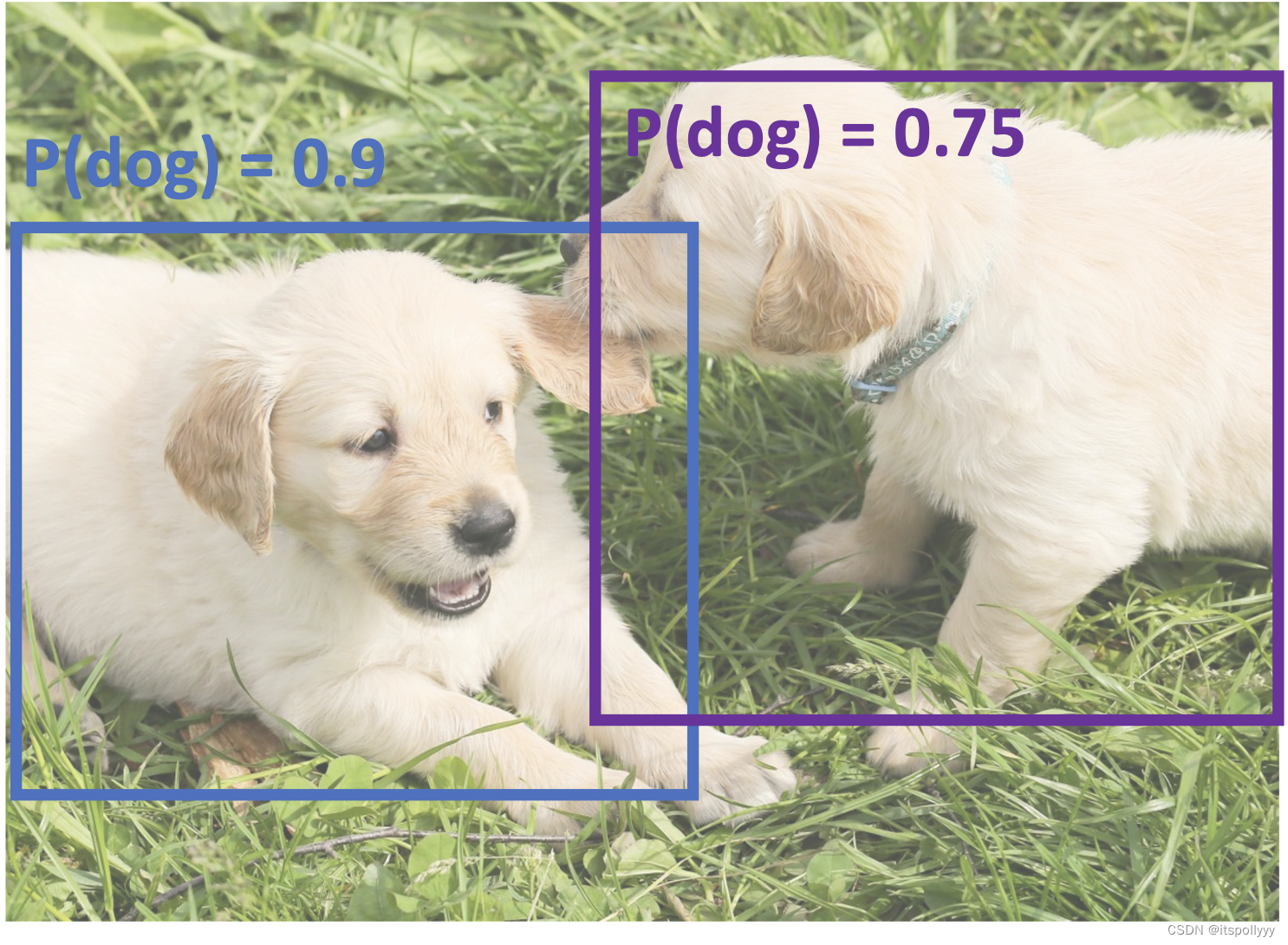
IoU(紫, 黄) = 0.74，得到紫框。

Reference：

1. 一阶目标检测（one-stage object detection）整理归纳

2.  FCOS: Fully Convolutional One-Stage Object Detection

3. FCOS: A Simple and Strong Anchor-free Object Detector

4. EECS 498-007 / 598-005Deep Learning for Computer Vision

5. Feature Pyramid Networks for Object Detection

6.  1.1.2 FPN结构详解

7. FCOS Walkthrough: The Fully Convolutional Approach to Object Detection 

8. FCOS网络解析 

9. Focal Loss for Dense Object Detection 

10. Overlapping Boxes: Non-Max Suppression (NMS)