


第八周 猫狗识别
- 🍨 本文为🔗365天深度学习训练营 中的学习记录博客
- 🍦 参考文章:365天深度学习训练营-第8周:猫狗识别(训练营内部成员可读)
- 🍖 原作者:K同学啊|接辅导、项目定制
● 难度:夯实基础⭐⭐
● 语言:Python3、TensorFlow2
● 时间:9月12-9月16日
🍺 要求:
了解model.train_on_batch()并运用
了解tqdm,并使用tqdm实现可视化进度条
🍻 拔高(可选):
本文代码中存在一个严重的BUG,请找出它并配以文字说明
猜测:
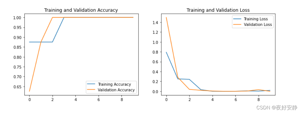
模型在训练过程中,第4个epoch,val_acc就达到了100%,这个有点诡异。猜测代码中的BUG引起的。感觉是训练数据和验证数据是同一份,用训练数据去做验证了,才能在如此短的时间内就达到了100%的val_acc,需要从这个方面去考虑修改代码。
🔎 探索(难度有点大)
修改代码,处理BUG
一、前期工作
1. 设置GPU
import tensorflow as tf

gpus = tf.config.list_physical_devices("GPU")
if gpus:
    tf.config.experimental.set_memory_growth(gpus[0], True)  #设置GPU显存用量按需使用
    tf.config.set_visible_devices([gpus[0]],"GPU")
gpus

2. 导入数据
# 2导入数据
import matplotlib.pyplot as plt
# 支持中文
plt.rcParams['font.sans-serif'] = ['SimHei']  # 用来正常显示中文标签
plt.rcParams['axes.unicode_minus'] = False  # 用来正常显示负号

import os,PIL,pathlib

#隐藏警告
import warnings
warnings.filterwarnings('ignore')

data_dir = "C:/study/artificialIntelligence/data/dog"
data_dir = pathlib.Path(data_dir)

image_count = len(list(data_dir.glob('*/*')))

print("图片总数为:",image_count)
image_count = len(list(data_dir.glob('*/*.png')))

print("图片总数为:",image_count)

二、数据预处理
1. 加载数据
使用image_dataset_from_directory方法将磁盘中的数据加载到tf.data.Dataset中
batch_size = 32
img_height = 224
img_width = 224
# 将文件夹中的数据加载到tf.data.Dataset中,且加载的同时会打乱数据。
train_ds = tf.keras.preprocessing.image_dataset_from_directory(
    data_dir,
    validation_split=0.2,
    subset='training',
    seed=123,
    batch_size=batch_size,
    image_size=(img_height,img_width)

)

函数原型
tf.keras.preprocessing.image_dataset_from_directory(
directory,
labels=“inferred”,
label_mode=“int”,
class_names=None,
color_mode=“rgb”,
batch_size=32,
image_size=(256, 256),
shuffle=True,
seed=None,
validation_split=None,
subset=None,
interpolation=“bilinear”,
follow_links=False,
)
参数
directory: 数据所在目录。如果标签是inferred(默认),则它应该包含子目录,每个目录包含一个类的图像。否则,将忽略目录结构。
labels: inferred(标签从目录结构生成),或者是整数标签的列表/元组,其大小与目录中找到的图像文件的数量相同。标签应根据图像文件路径的字母顺序排序(通过Python中的os.walk(directory)获得)。
label_mode:
int:标签将被编码成整数(使用的损失函数应为:sparse_categorical_crossentropy loss)。
categorical:标签将被编码为分类向量(使用的损失函数应为:categorical_crossentropy loss)。
binary:意味着标签(只能有2个)被编码为值为0或1的float32标量(例如:binary_crossentropy)。
None:(无标签)。
class_names: 仅当labels为inferred时有效。这是类名称的明确列表(必须与子目录的名称匹配)。用于控制类的顺序(否则使用字母数字顺序)。
color_mode: grayscale、rgb、rgba之一。默认值:rgb。图像将被转换为1、3或者4通道。
batch_size: 数据批次的大小。默认值:32
image_size: 从磁盘读取数据后将其重新调整大小。默认:(256,256)。由于管道处理的图像批次必须具有相同的大小,因此该参数必须提供。
shuffle: 是否打乱数据。默认值:True。如果设置为False,则按字母数字顺序对数据进行排序。
seed: 用于shuffle和转换的可选随机种子。
validation_split: 0和1之间的可选浮点数,可保留一部分数据用于验证。
subset: training或validation之一。仅在设置validation_split时使用。
interpolation: 字符串,当调整图像大小时使用的插值方法。默认为:bilinear。支持bilinear, nearest, bicubic, area, lanczos3, lanczos5, gaussian, mitchellcubic。
follow_links: 是否访问符号链接指向的子目录。默认:False。
val_ds = tf.keras.preprocessing.image_dataset_from_directory(
    data_dir,
    validation_split=0.2,
    subset='validation',
    seed=123,
    batch_size=batch_size,
    image_size=(img_height, img_width)

)

我们可以通过class_names输出数据集的标签。标签将按字母顺序对应于目录名称。
class_names = train_ds.class_names
print(class_names)

3.配置数据集
● shuffle() :打乱数据,关于此函数的详细介绍可以参考:https://zhuanlan.zhihu.com/p/42417456
● prefetch() :预取数据,加速运行,其详细介绍可以参考我前两篇文章,里面都有讲解。
● cache() :将数据集缓存到内存当中,加速运行
AUTOTUNE = tf.data.AUTOTUNE

def preprocess_image(image,label):
    return (image/255.0,label)

# 归一化处理
train_ds = train_ds.map(preprocess_image, num_parallel_calls=AUTOTUNE)
val_ds   = val_ds.map(preprocess_image, num_parallel_calls=AUTOTUNE)

train_ds = train_ds.cache().shuffle(1000).prefetch(buffer_size=AUTOTUNE)
val_ds   = val_ds.cache().prefetch(buffer_size=AUTOTUNE)

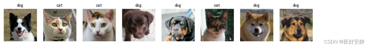
4.可视化数据
plt.figure(figsize=(15, 10))  # 图形的宽为15高为10

for images, labels in train_ds.take(1):
    for i in range(8):

        ax = plt.subplot(5, 8, i + 1)
        plt.imshow(images[i])
        plt.title(class_names[labels[i]])

        plt.axis("off")
三、构建VGG-16网络
VGG优缺点分析:
● VGG优点
VGG的结构非常简洁,整个网络都使用了同样大小的卷积核尺寸(3x3)和最大池化尺寸(2x2)。
● VGG缺点
1)训练时间过长,调参难度大。2)需要的存储容量大,不利于部署。例如存储VGG-16权重值文件的大小为500多MB,不利于安装到嵌入式系统中。
自建模型
from tensorflow.keras import layers, models, Input
from tensorflow.keras.models import Model
from tensorflow.keras.layers import Conv2D, MaxPooling2D, Dense, Flatten, Dropout

def VGG16(nb_classes, input_shape):
    input_tensor = Input(shape=input_shape)
    # 1st block
    x = Conv2D(64, (3,3), activation='relu', padding='same',name='block1_conv1')(input_tensor)
    x = Conv2D(64, (3,3), activation='relu', padding='same',name='block1_conv2')(x)
    x = MaxPooling2D((2,2), strides=(2,2), name = 'block1_pool')(x)
    # 2nd block
    x = Conv2D(128, (3,3), activation='relu', padding='same',name='block2_conv1')(x)
    x = Conv2D(128, (3,3), activation='relu', padding='same',name='block2_conv2')(x)
    x = MaxPooling2D((2,2), strides=(2,2), name = 'block2_pool')(x)
    # 3rd block
    x = Conv2D(256, (3,3), activation='relu', padding='same',name='block3_conv1')(x)
    x = Conv2D(256, (3,3), activation='relu', padding='same',name='block3_conv2')(x)
    x = Conv2D(256, (3,3), activation='relu', padding='same',name='block3_conv3')(x)
    x = MaxPooling2D((2,2), strides=(2,2), name = 'block3_pool')(x)
    # 4th block
    x = Conv2D(512, (3,3), activation='relu', padding='same',name='block4_conv1')(x)
    x = Conv2D(512, (3,3), activation='relu', padding='same',name='block4_conv2')(x)
    x = Conv2D(512, (3,3), activation='relu', padding='same',name='block4_conv3')(x)
    x = MaxPooling2D((2,2), strides=(2,2), name = 'block4_pool')(x)
    # 5th block
    x = Conv2D(512, (3,3), activation='relu', padding='same',name='block5_conv1')(x)
    x = Conv2D(512, (3,3), activation='relu', padding='same',name='block5_conv2')(x)
    x = Conv2D(512, (3,3), activation='relu', padding='same',name='block5_conv3')(x)
    x = MaxPooling2D((2,2), strides=(2,2), name = 'block5_pool')(x)
    # full connection
    x = Flatten()(x)
    x = Dense(4096, activation='relu',  name='fc1')(x)
    x = Dense(4096, activation='relu', name='fc2')(x)
    output_tensor = Dense(nb_classes, activation='softmax', name='predictions')(x)

    model = Model(input_tensor, output_tensor)
    return model

model=VGG16(1000, (img_width, img_height, 3))
model.summary()
Model: "model"
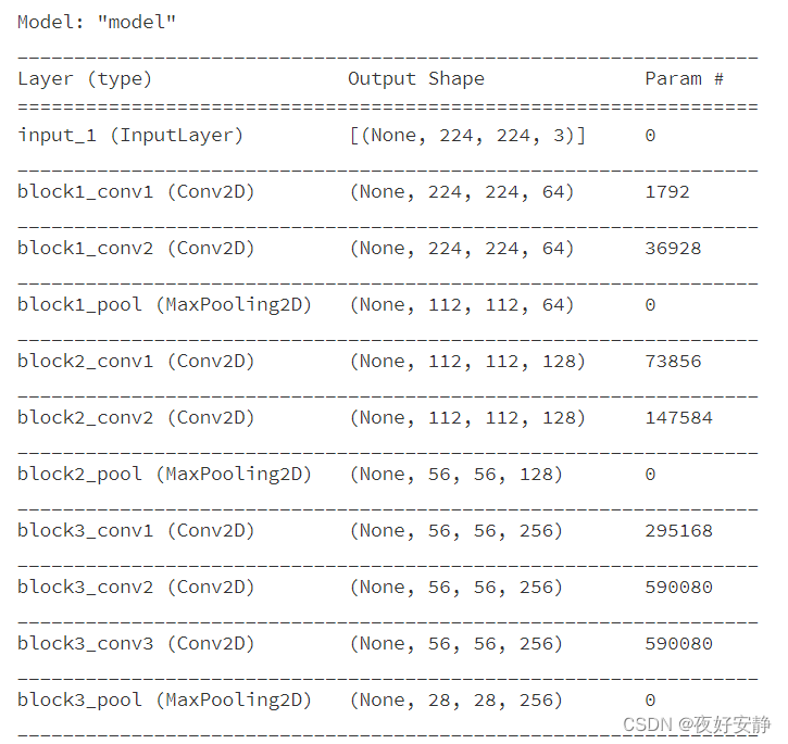
网络结构
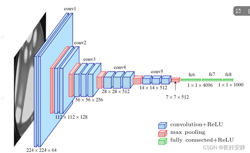
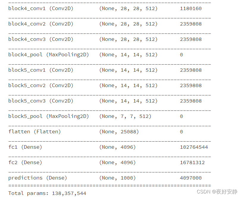
结构说明:
● 13个卷积层(Convolutional Layer),分别用blockX_convX表示
● 3个全连接层(Fully connected Layer),分别用fcX与predictions表示
● 5个池化层(Pool layer),分别用blockX_pool表示
VGG-16包含了16个隐藏层(13个卷积层和3个全连接层,具有激活函数),故称为VGG-16
四、编译
在准备对模型进行训练之前,还需要再对其进行一些设置。以下内容是在模型的编译步骤中添加的:
● 损失函数(loss):用于衡量模型在训练期间的准确率。
● 优化器(optimizer):决定模型如何根据其看到的数据和自身的损失函数进行更新。
● 指标(metrics):用于监控训练和测试步骤。以下示例使用了准确率,即被正确分类的图像的比率。
model.compile(optimizer="adam",
              loss     ='sparse_categorical_crossentropy',
              metrics  =['accuracy'])
五、训练模型
from tqdm import tqdm
import tensorflow.keras.backend as K

epochs = 10
lr     = 1e-4

# 记录训练数据,方便后面的分析
history_train_loss     = []
history_train_accuracy = []
history_val_loss       = []
history_val_accuracy   = []

for epoch in range(epochs):
    train_total = len(train_ds)
    val_total   = len(val_ds)

    """
    total:预期的迭代数目
    ncols:控制进度条宽度
    mininterval:进度更新最小间隔,以秒为单位(默认值:0.1)
    """
    with tqdm(total=train_total, desc=f'Epoch {epoch + 1}/{epochs}',mininterval=1,ncols=100) as pbar:

        lr = lr*0.92
        K.set_value(model.optimizer.lr, lr)

        for image,label in train_ds:
            """
            训练模型,简单理解train_on_batch就是:它是比model.fit()更高级的一个用法

            想详细了解 train_on_batch 的同学,
            可以看看我的这篇文章:https://www.yuque.com/mingtian-fkmxf/hv4lcq/ztt4gy
            """
            history = model.train_on_batch(image,label)

            train_loss     = history[0]
            train_accuracy = history[1]

            pbar.set_postfix({"loss": "%.4f"%train_loss,
                              "accuracy":"%.4f"%train_accuracy,
                              "lr": K.get_value(model.optimizer.lr)})
            pbar.update(1)
        history_train_loss.append(train_loss)
        history_train_accuracy.append(train_accuracy)

    print('开始验证!')

    with tqdm(total=val_total, desc=f'Epoch {epoch + 1}/{epochs}',mininterval=0.3,ncols=100) as pbar:

        for image,label in val_ds:

            history = model.test_on_batch(image,label)

            val_loss     = history[0]
            val_accuracy = history[1]

            pbar.set_postfix({"loss": "%.4f"%val_loss,
                              "accuracy":"%.4f"%val_accuracy})
            pbar.update(1)
        history_val_loss.append(val_loss)
        history_val_accuracy.append(val_accuracy)

    print('结束验证!')
    print("验证loss为:%.4f"%val_loss)
    print("验证准确率为:%.4f"%val_accuracy)

六、模型评估
epochs_range = range(epochs)

plt.figure(figsize=(12, 4))
plt.subplot(1, 2, 1)

plt.plot(epochs_range, history_train_accuracy, label='Training Accuracy')
plt.plot(epochs_range, history_val_accuracy, label='Validation Accuracy')
plt.legend(loc='lower right')
plt.title('Training and Validation Accuracy')

plt.subplot(1, 2, 2)
plt.plot(epochs_range, history_train_loss, label='Training Loss')
plt.plot(epochs_range, history_val_loss, label='Validation Loss')
plt.legend(loc='upper right')
plt.title('Training and Validation Loss')
plt.show()


 1010
1010


 被折叠的 条评论
为什么被折叠?
被折叠的 条评论
为什么被折叠?
 到【灌水乐园】发言


