理解sklearn决策树的clf.tree_结构（适用于随机森林）

一直想看看tree_到底是怎么个结构，搜索也没有个详细的讲解，在参考了官方文档后（没有我的详细，主要是讲怎么绘制路径的），自己试了挺久终于搞懂了。

下面用随机森林的例子开始：RandomForestClassifier中的每棵树都相当于DecisionTreeClassifier的实例。

---

from sklearn.model_selection import train_test_split, cross_val_score, KFold, GridSearchCV
import pandas as pd
import numpy as np

from sklearn.ensemble import RandomForestClassifier
from sklearn.metrics import accuracy_score, make_scorer
from sklearn.metrics import confusion_matrix
from sklearn.metrics import classification_report
from sklearn.preprocessing import StandardScaler

from sklearn.datasets import load_breast_cancer
from sklearn.ensemble import RandomForestClassifier
from sklearn.model_selection import cross_val_score
from sklearn.model_selection import GridSearchCV
import numpy as np
from numpy import mat
import pandas as pd
import matplotlib.pyplot as plt

from tqdm import tqdm

"""测试一下一般情况下（未调参）的得分"""

# 导入乳腺癌数据集
data = load_breast_cancer()
data

{'data': array([[1.799e+01, 1.038e+01, 1.228e+02, ..., 2.654e-01, 4.601e-01,
        1.189e-01],
       [2.057e+01, 1.777e+01, 1.329e+02, ..., 1.860e-01, 2.750e-01,
        8.902e-02],
       [1.969e+01, 2.125e+01, 1.300e+02, ..., 2.430e-01, 3.613e-01,
        8.758e-02],
       ...,
       [1.660e+01, 2.808e+01, 1.083e+02, ..., 1.418e-01, 2.218e-01,
        7.820e-02],
       [2.060e+01, 2.933e+01, 1.401e+02, ..., 2.650e-01, 4.087e-01,
        1.240e-01],
       [7.760e+00, 2.454e+01, 4.792e+01, ..., 0.000e+00, 2.871e-01,
        7.039e-02]]),
'target': array([0, 0, 0, 0, 0, 0, 0, 0, 0, 0, 0, 0, 0, 0, 0, 0, 0, 0, 0, 1, 1, 1,
       0, 0, 0, 0, 0, 0, 0, 0, 0, 0, 0, 0, 0, 0, 0, 1, 0, 0, 0, 0, 0, 0,
       0, 0, 1, 0, 1, 1, 1, 1, 1, 0, 0, 1, 0, 0, 1, 1, 1, 1, 0, 1, 0, 0,
       1, 1, 1, 1, 0, 1, 0, 0, 1, 0, 1, 0, 0, 1, 1, 1, 0, 0, 1, 0, 0, 0,
       1, 1, 1, 0, 1, 1, 0, 0, 1, 1, 1, 0, 0, 1, 1, 1, 1, 0, 1, 1, 0, 1,
       1, 1, 1, 1, 1, 1, 1, 0, 0, 0, 1, 0, 0, 1, 1, 1, 0, 0, 1, 0, 1, 0,
       0, 1, 0, 0, 1, 1, 0, 1, 1, 0, 1, 1, 1, 1, 0, 1, 1, 1, 1, 1, 1, 1,
       1, 1, 0, 1, 1, 1, 1, 0, 0, 1, 0, 1, 1, 0, 0, 1, 1, 0, 0, 1, 1, 1,
       1, 0, 1, 1, 0, 0, 0, 1, 0, 1, 0, 1, 1, 1, 0, 1, 1, 0, 0, 1, 0, 0,
       0, 0, 1, 0, 0, 0, 1, 0, 1, 0, 1, 1, 0, 1, 0, 0, 0, 0, 1, 1, 0, 0,
       1, 1, 1, 0, 1, 1, 1, 1, 1, 0, 0, 1, 1, 0, 1, 1, 0, 0, 1, 0, 1, 1,
       1, 1, 0, 1, 1, 1, 1, 1, 0, 1, 0, 0, 0, 0, 0, 0, 0, 0, 0, 0, 0, 0,
       0, 0, 1, 1, 1, 1, 1, 1, 0, 1, 0, 1, 1, 0, 1, 1, 0, 1, 0, 0, 1, 1,
       1, 1, 1, 1, 1, 1, 1, 1, 1, 1, 1, 0, 1, 1, 0, 1, 0, 1, 1, 1, 1, 1,
       1, 1, 1, 1, 1, 1, 1, 1, 1, 0, 1, 1, 1, 0, 1, 0, 1, 1, 1, 1, 0, 0,
       0, 1, 1, 1, 1, 0, 1, 0, 1, 0, 1, 1, 1, 0, 1, 1, 1, 1, 1, 1, 1, 0,
       0, 0, 1, 1, 1, 1, 1, 1, 1, 1, 1, 1, 1, 0, 0, 1, 0, 0, 0, 1, 0, 0,
       1, 1, 1, 1, 1, 0, 1, 1, 1, 1, 1, 0, 1, 1, 1, 0, 1, 1, 0, 0, 1, 1,
       1, 1, 1, 1, 0, 1, 1, 1, 1, 1, 1, 1, 0, 1, 1, 1, 1, 1, 0, 1, 1, 0,
       1, 1, 1, 1, 1, 1, 1, 1, 1, 1, 1, 1, 0, 1, 0, 0, 1, 0, 1, 1, 1, 1,
       1, 0, 1, 1, 0, 1, 0, 1, 1, 0, 1, 0, 1, 1, 1, 1, 1, 1, 1, 1, 0, 0,
       1, 1, 1, 1, 1, 1, 0, 1, 1, 1, 1, 1, 1, 1, 1, 1, 1, 0, 1, 1, 1, 1,
       1, 1, 1, 0, 1, 0, 1, 1, 0, 1, 1, 1, 1, 1, 0, 0, 1, 0, 1, 0, 1, 1,
       1, 1, 1, 0, 1, 1, 0, 1, 0, 1, 0, 0, 1, 1, 1, 0, 1, 1, 1, 1, 1, 1,
       1, 1, 1, 1, 1, 0, 1, 0, 0, 1, 1, 1, 1, 1, 1, 1, 1, 1, 1, 1, 1, 1,
       1, 1, 1, 1, 1, 1, 1, 1, 1, 1, 1, 1, 0, 0, 0, 0, 0, 0, 1]),
'target_names': array(['malignant', 'benign'], dtype='<U9'),
'DESCR': '.. _breast_cancer_dataset:\n\nBreast cancer wisconsin (diagnostic) dataset\n--------------------------------------------\n\n**Data Set Characteristics:**\n\n    :Number of Instances: 569\n\n    :Number of Attributes: 30 numeric, predictive attributes and the class\n\n    :Attribute Information:\n        - radius (mean of distances from center to points on the perimeter)\n        - texture (standard deviation of gray-scale values)\n        - perimeter\n        - area\n        - smoothness (local variation in radius lengths)\n        - compactness (perimeter^2 / area - 1.0)\n        - concavity (severity of concave portions of the contour)\n        - concave points (number of concave portions of the contour)\n        - symmetry \n        - fractal dimension ("coastline approximation" - 1)\n\n        The mean, standard error, and "worst" or largest (mean of the three\n        largest values) of these features were computed for each image,\n        resulting in 30 features.  For instance, field 3 is Mean Radius, field\n        13 is Radius SE, field 23 is Worst Radius.\n\n        - class:\n                - WDBC-Malignant\n                - WDBC-Benign\n\n    :Summary Statistics:\n\n    ===================================== ====== ======\n                                           Min    Max\n    ===================================== ====== ======\n    radius (mean):                        6.981  28.11\n    texture (mean):                       9.71   39.28\n    perimeter (mean):                     43.79  188.5\n    area (mean):                          143.5  2501.0\n    smoothness (mean):                    0.053  0.163\n    compactness (mean):                   0.019  0.345\n    concavity (mean):                     0.0    0.427\n    concave points (mean):                0.0    0.201\n    symmetry (mean):                      0.106  0.304\n    fractal dimension (mean):             0.05   0.097\n    radius (standard error):              0.112  2.873\n    texture (standard error):             0.36   4.885\n    perimeter (standard error):           0.757  21.98\n    area (standard error):                6.802  542.2\n    smoothness (standard error):          0.002  0.031\n    compactness (standard error):         0.002  0.135\n    concavity (standard error):           0.0    0.396\n    concave points (standard error):      0.0    0.053\n    symmetry (standard error):            0.008  0.079\n    fractal dimension (standard error):   0.001  0.03\n    radius (worst):                       7.93   36.04\n    texture (worst):                      12.02  49.54\n    perimeter (worst):                    50.41  251.2\n    area (worst):                         185.2  4254.0\n    smoothness (worst):                   0.071  0.223\n    compactness (worst):                  0.027  1.058\n    concavity (worst):                    0.0    1.252\n    concave points (worst):               0.0    0.291\n    symmetry (worst):                     0.156  0.664\n    fractal dimension (worst):            0.055  0.208\n    ===================================== ====== ======\n\n    :Missing Attribute Values: None\n\n    :Class Distribution: 212 - Malignant, 357 - Benign\n\n    :Creator:  Dr. William H. Wolberg, W. Nick Street, Olvi L. Mangasarian\n\n    :Donor: Nick Street\n\n    :Date: November, 1995\n\nThis is a copy of UCI ML Breast Cancer Wisconsin (Diagnostic) datasets.\nhttps://goo.gl/U2Uwz2\n\nFeatures are computed from a digitized image of a fine needle\naspirate (FNA) of a breast mass.  They describe\ncharacteristics of the cell nuclei present in the image.\n\nSeparating plane described above was obtained using\nMultisurface Method-Tree (MSM-T) [K. P. Bennett, "Decision Tree\nConstruction Via Linear Programming." Proceedings of the 4th\nMidwest Artificial Intelligence and Cognitive Science Society,\npp. 97-101, 1992], a classification method which uses linear\nprogramming to construct a decision tree.  Relevant features\nwere selected using an exhaustive search in the space of 1-4\nfeatures and 1-3 separating planes.\n\nThe actual linear program used to obtain the separating plane\nin the 3-dimensional space is that described in:\n[K. P. Bennett and O. L. Mangasarian: "Robust Linear\nProgramming Discrimination of Two Linearly Inseparable Sets",\nOptimization Methods and Software 1, 1992, 23-34].\n\nThis database is also available through the UW CS ftp server:\n\nftp ftp.cs.wisc.edu\ncd math-prog/cpo-dataset/machine-learn/WDBC/\n\n.. topic:: References\n\n   - W.N. Street, W.H. Wolberg and O.L. Mangasarian. Nuclear feature extraction \n     for breast tumor diagnosis. IS&T/SPIE 1993 International Symposium on \n     Electronic Imaging: Science and Technology, volume 1905, pages 861-870,\n     San Jose, CA, 1993.\n   - O.L. Mangasarian, W.N. Street and W.H. Wolberg. Breast cancer diagnosis and \n     prognosis via linear programming. Operations Research, 43(4), pages 570-577, \n     July-August 1995.\n   - W.H. Wolberg, W.N. Street, and O.L. Mangasarian. Machine learning techniques\n     to diagnose breast cancer from fine-needle aspirates. Cancer Letters 77 (1994) \n     163-171.',
'feature_names': array(['mean radius', 'mean texture', 'mean perimeter', 'mean area',
       'mean smoothness', 'mean compactness', 'mean concavity',
       'mean concave points', 'mean symmetry', 'mean fractal dimension',
       'radius error', 'texture error', 'perimeter error', 'area error',
       'smoothness error', 'compactness error', 'concavity error',
       'concave points error', 'symmetry error',
       'fractal dimension error', 'worst radius', 'worst texture',
       'worst perimeter', 'worst area', 'worst smoothness',
       'worst compactness', 'worst concavity', 'worst concave points',
       'worst symmetry', 'worst fractal dimension'], dtype='<U23'),
'filename': 'C:\\Users\\xia\\AppData\\Roaming\\Python\\Python37\\site-packages\\sklearn\\datasets\\data\\breast_cancer.csv'}

# 划分训练集和测试集
X_train, X_test, Y_train, Y_test = train_test_split(data.data, 
                                                    data.target,
                                                    test_size=0.2, 
                                                    random_state=0)

# 构建随机森林模型，拟合训练
rfc = RandomForestClassifier(oob_score=True, 
                             n_estimators=44, 
                             random_state=90, 
                             n_jobs=4)
clf = rfc.fit(X_train,Y_train)

# 查看OOB分数
clf.oob_score_

0.9538461538461539

# 第0棵树
tree_0 = clf.estimators_[0]    

# 将决策树绘制成图到你当前的路径

from sklearn.tree import export_text, export_graphviz
# 加入Graphviz的环境路径
import os
os.environ["PATH"] += os.pathsep + "G:/24_graphviz_msi/bin"

# 绘图并导出
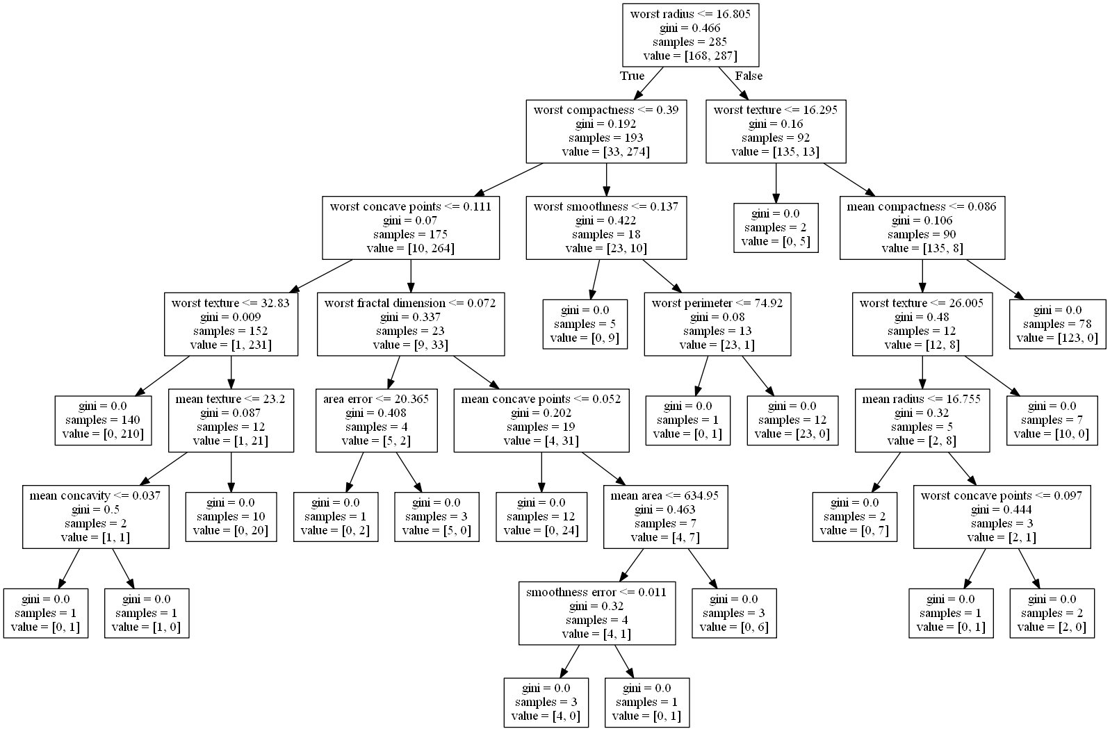
dot_data = export_graphviz(tree_0, out_file=None,
                           feature_names=data.feature_names)
import pydotplus

graph = pydotplus.graph_from_dot_data(dot_data)
graph.get_nodes()[7].set_fillcolor("#FFF2DD")
if os.path.exists("out_0.png"):
   pass
else:
    graph.write_png("out_0.png")  # 当前文件夹生成out.png

为了快速演示，这里也展示一下图

# 查看第0棵树的各项信息
n_nodes = tree_0.tree_.node_count
print(f"n_nodes = {n_nodes}\n")

children_left = tree_0.tree_.children_left  # 左子节点的id，-1代表其parent无左子节点
print(f"children_left = {children_left}\n") # 右子节点的id，-1代表其parent无子节点

children_right = tree_0.tree_.children_right
print(f"children_right = {children_right}\n")

features = tree_0.tree_.feature     # 特征所在序号
print(f"features = {features}\n")

threshold = tree_0.tree_.threshold  # 特征的切分阈值
print(f"threshold = {threshold}\n")

feature_names = data.feature_names  # 数据的特征名
print(f"features_names = {feature_names}")

n_nodes = 37

children_left = [ 1  2  3  4 -1  6  7 -1 -1 -1 11 12 -1 -1 15 -1 17 18 -1 -1 -1 22 -1 24
 -1 -1 27 -1 29 30 31 -1 33 -1 -1 -1 -1]

children_right = [26 21 10  5 -1  9  8 -1 -1 -1 14 13 -1 -1 16 -1 20 19 -1 -1 -1 23 -1 25
 -1 -1 28 -1 36 35 32 -1 34 -1 -1 -1 -1]

features = [20 25 27 21 -2  1  6 -2 -2 -2 29 13 -2 -2  7 -2  3 14 -2 -2 -2 24 -2 22
 -2 -2 21 -2  5 21  0 -2 27 -2 -2 -2 -2]

threshold = [ 1.68050003e+01  3.90100002e-01  1.10849999e-01  3.28299999e+01
 -2.00000000e+00  2.31999998e+01  3.74699989e-02 -2.00000000e+00
 -2.00000000e+00 -2.00000000e+00  7.20250010e-02  2.03650007e+01
 -2.00000000e+00 -2.00000000e+00  5.15999999e-02 -2.00000000e+00
  6.34949982e+02  1.13269999e-02 -2.00000000e+00 -2.00000000e+00
 -2.00000000e+00  1.36700004e-01 -2.00000000e+00  7.49200020e+01
 -2.00000000e+00 -2.00000000e+00  1.62950001e+01 -2.00000000e+00
  8.55550021e-02  2.60050001e+01  1.67550001e+01 -2.00000000e+00
  9.65050012e-02 -2.00000000e+00 -2.00000000e+00 -2.00000000e+00
 -2.00000000e+00]

features_names = ['mean radius' 'mean texture' 'mean perimeter' 'mean area'
 'mean smoothness' 'mean compactness' 'mean concavity'
 'mean concave points' 'mean symmetry' 'mean fractal dimension'
 'radius error' 'texture error' 'perimeter error' 'area error'
 'smoothness error' 'compactness error' 'concavity error'
 'concave points error' 'symmetry error' 'fractal dimension error'
 'worst radius' 'worst texture' 'worst perimeter' 'worst area'
 'worst smoothness' 'worst compactness' 'worst concavity'
 'worst concave points' 'worst symmetry' 'worst fractal dimension']

先别急着自己尝试去看懂上面几串列表什么意思！

接着往下再看看

feature_names[20]

'worst radius'

# 查看id=0的节点左/右子节点是什么
print(children_left[0])
print(children_right[0])

1
26

# 查看id=1的节点左/右子节点是什么
print(children_left[4])
print(children_right[4])

-1
-1

# 查看id=32的节点左/右子节点是什么
print(children_left[32])
print(children_right[32])

33
34

根据上面的out.png和输出结果，可以发现：

1、对于节点数组left和right，-1表示叶节点

2、对于阈值threshold，-2表示叶节点的特征阈值

3、图上的数值是保留了3位小数的浮点数结果

4、left数组是根节点（不含根节点本身）左子树前序遍历的节点id序列（含叶节点）

5、right数组是根节点（不含根节点本身）的右子树前序遍历的节点id序列（含叶节点）

6、threshold和features的顺序就是left——>right顺序

为了方便快速理解，我加了些标注

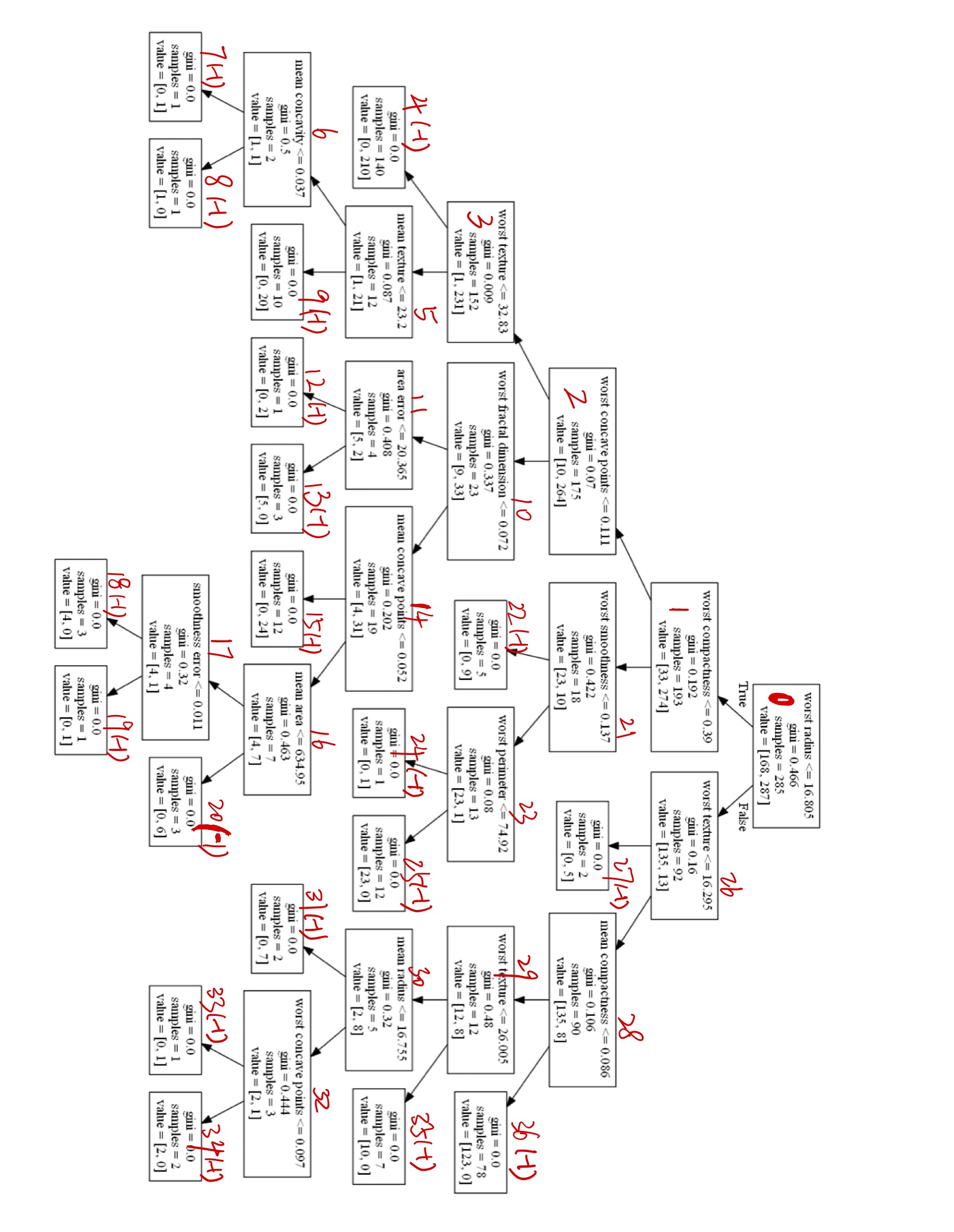
最后举个例子，在先序遍历完id=8的节点后，回到id=5的节点，此时可以找到right_child[5] = 9

OK，到此，tree_的结构就差不多了，可以用来应付很多问题了

参考：
官方文档《Understanding the decision tree structure》