


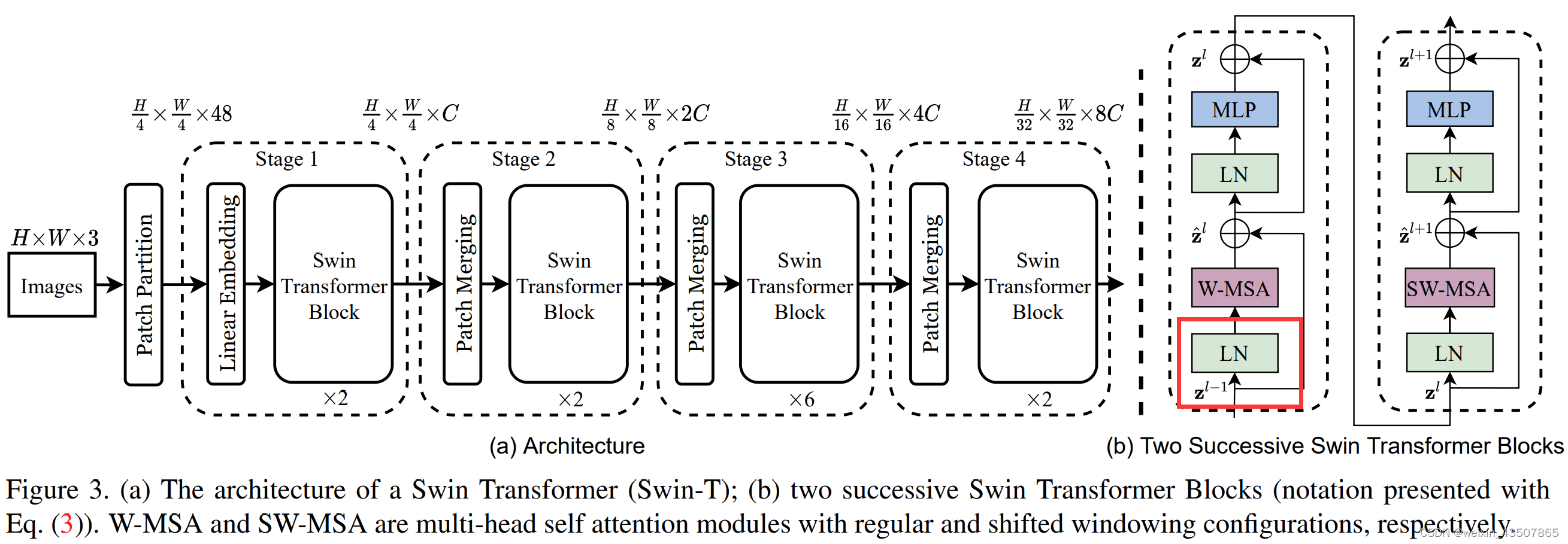
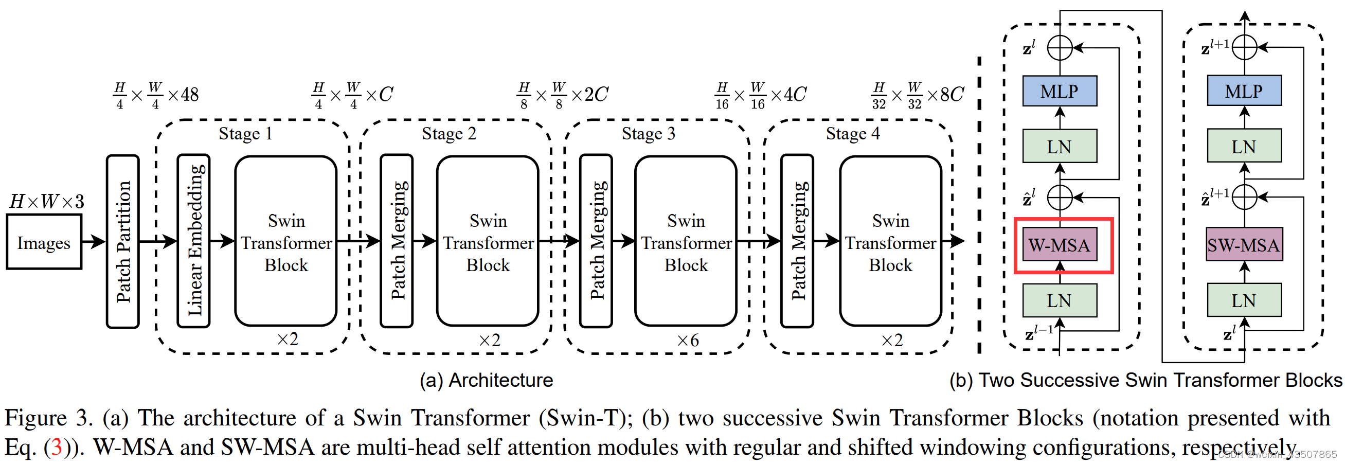
 本文详细解析了SwinTransformer模型中的关键组件,包括PatchEmbedding、W-MSA和SW-MSA模块,以及如何通过窗口划分、相对位置编码和注意力机制来实现高效的图像处理。文章还介绍了PatchMerging过程,展示了模型如何逐步处理并合并特征。
论文地址:https://arxiv.org/pdf/2103.14030.pdf
模型原理:Swin-Transformer网络结构详解_swin transformer-CSDN博客
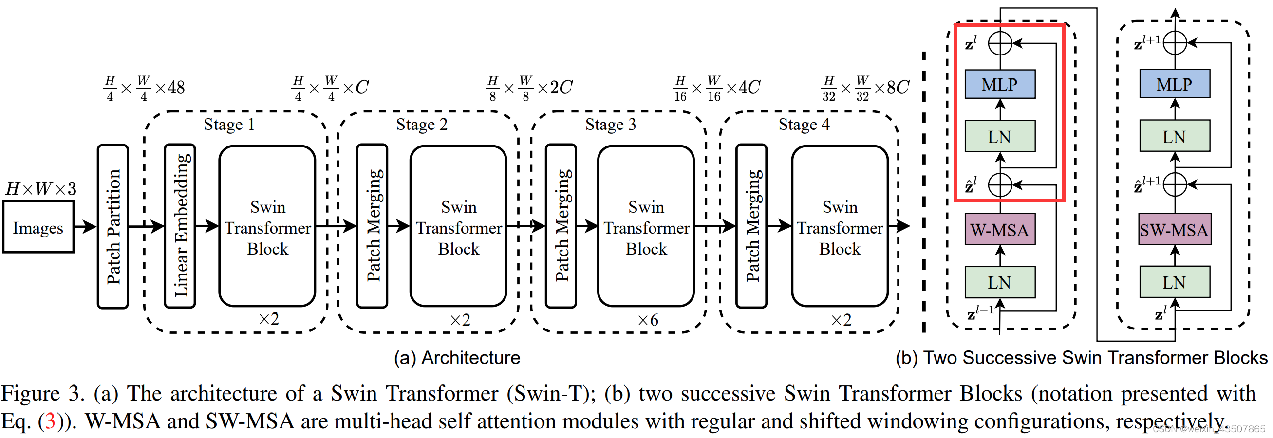
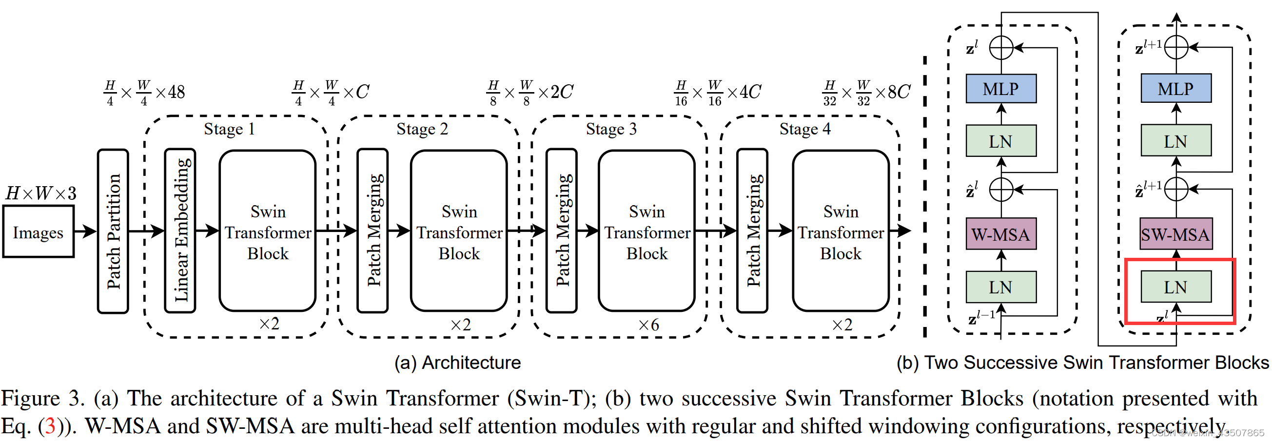
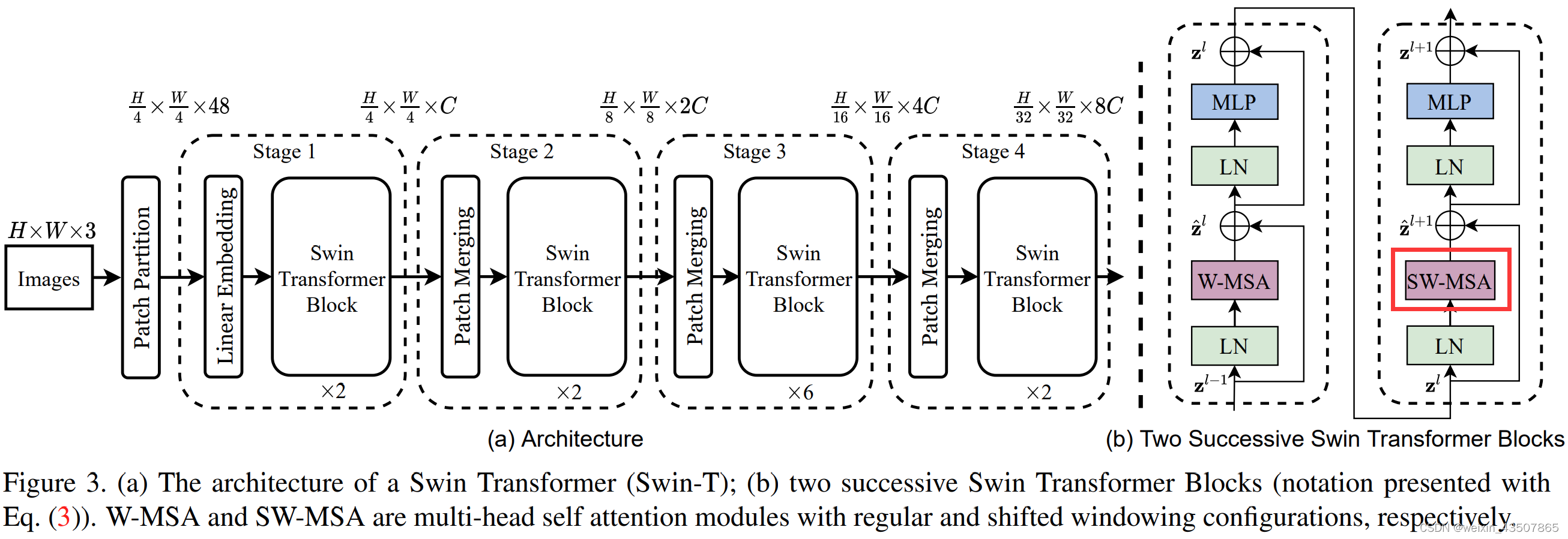
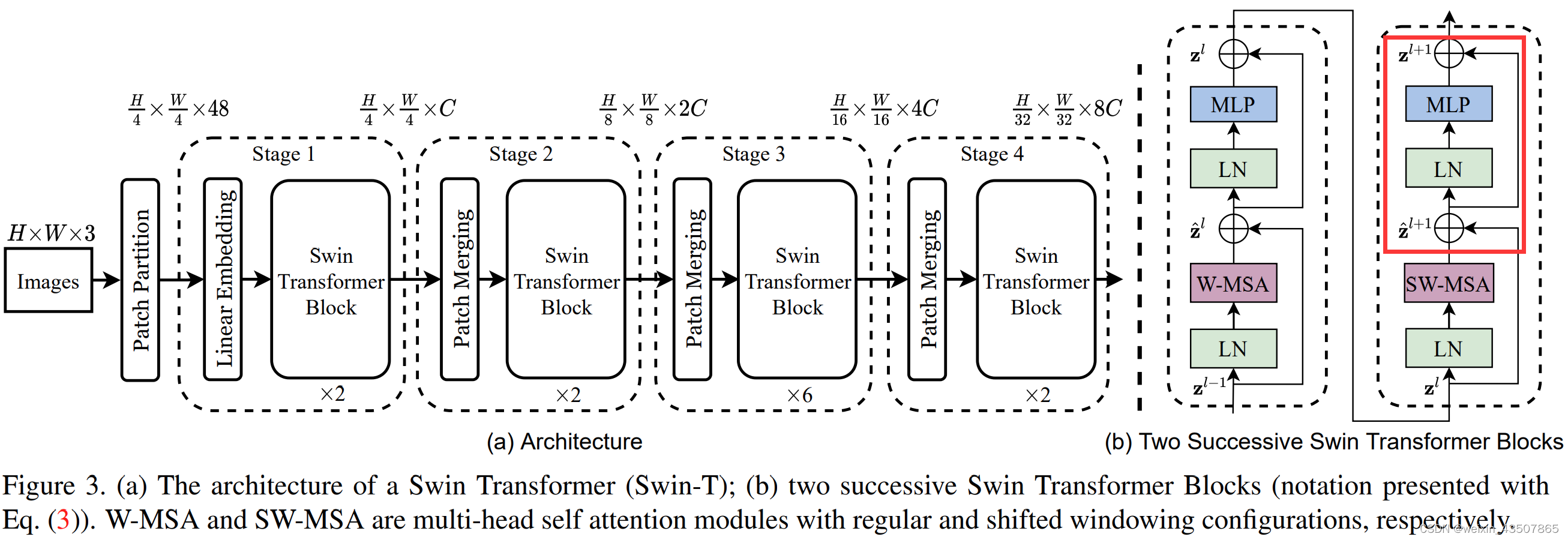
1. 整体流程图
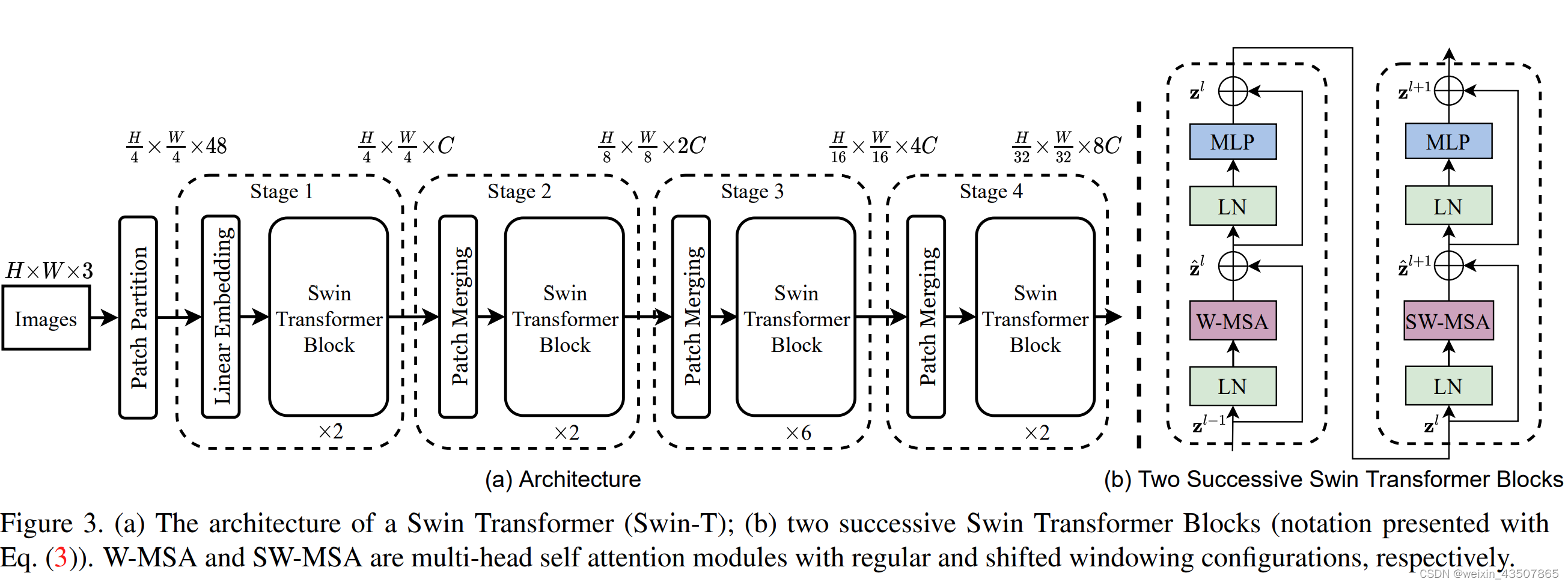
2. PatchEmbedding
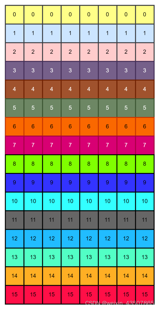
输入:预处理之后的原始图像(这里为了演示方便,将每张图像缩放成 16*16*3,每个批次为 2,因此输入的维度是(2, 3, 16, 16))
处理:nn.Conv2d
输出:(2, 16, 8)
在源码中,实际上就是一个卷积操作。 x = self.proj(x),self.proj = nn.Conv2d(in_c, embed_dim, kernel_size=patch_size, stride=patch_size)
输入 x 的 shape 为(B, C, H, W),输出 x 的 shape 为(B, C, H, W)。假设输入 x 的 shape 为(2,3,16,16),那么输出 x 的 shape 为(2,8,4,4)。
在卷积操作之后,还需要对形状做一次变形。x = x.flatten(2).transpose(1, 2),假设输入 x 的 shape 为(2,8,4,4),那么输出 x 的 shape 为(2,16,8)。如下图所示:
3. SwinTransformerBlock
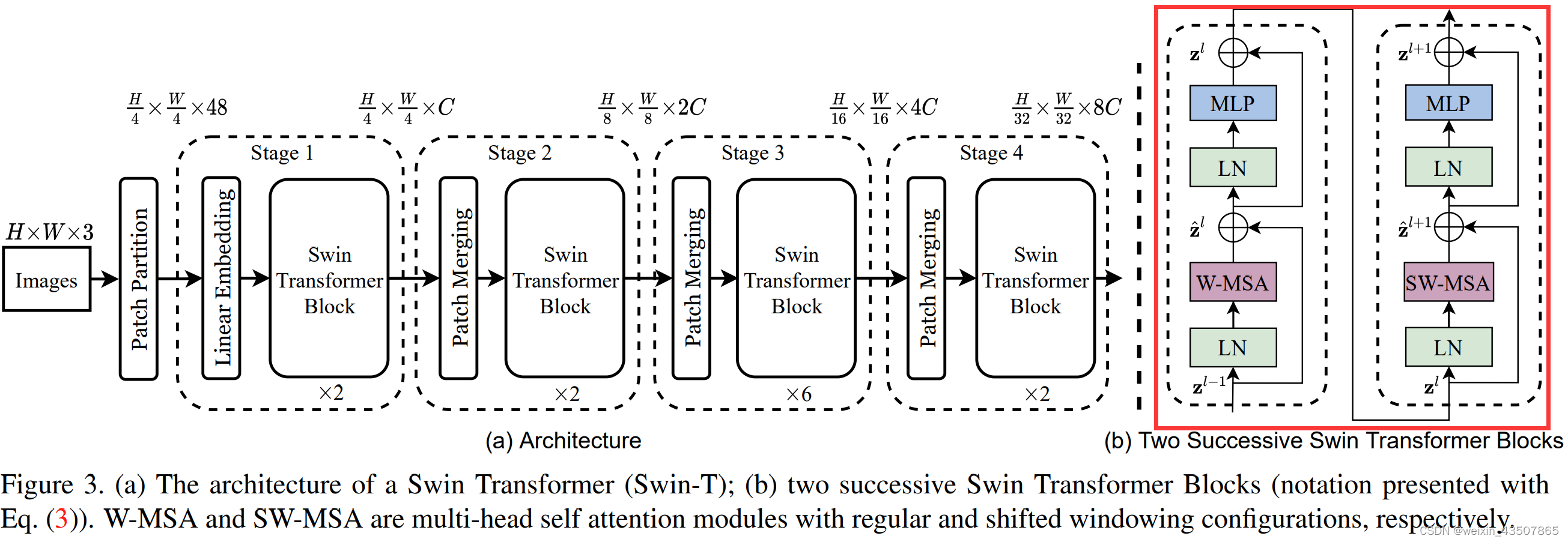
3.1. W-MSA 部分中的第一个 LN 层
输入:PatchEmbedding 的输出,即(2, 16, 8)
处理:nn.LayerNorm
输出:(2, 4, 4, 8)
x = self.norm1(x) # 层标准化
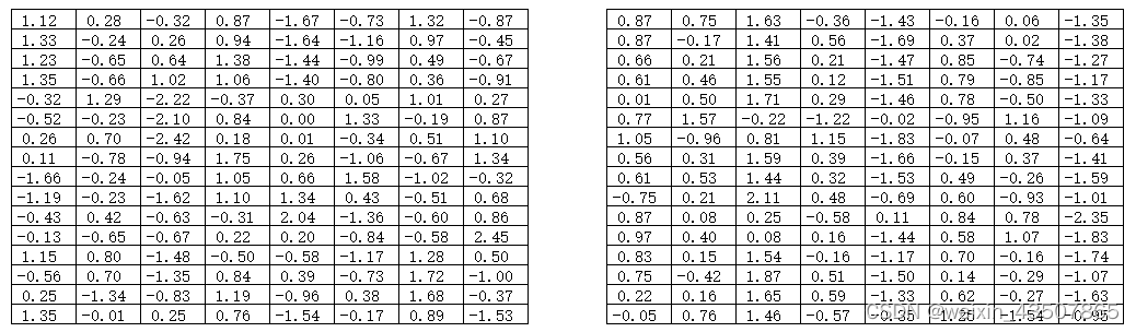
x = x.view(B, H, W, C) # 改变tensor形状,(2, 4, 4, 8)x = self.norm1(x)的结果如下:
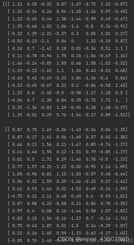
x = x.view(B, H, W, C)的结果如下:
3.2. W-MSA
先对 x 进行重构
# 把feature map给pad到window size的整数倍
pad_l = pad_t = 0
pad_r = (self.window_size - W % self.window_size) % self.window_size
pad_b = (self.window_size - H % self.window_size) % self.window_size
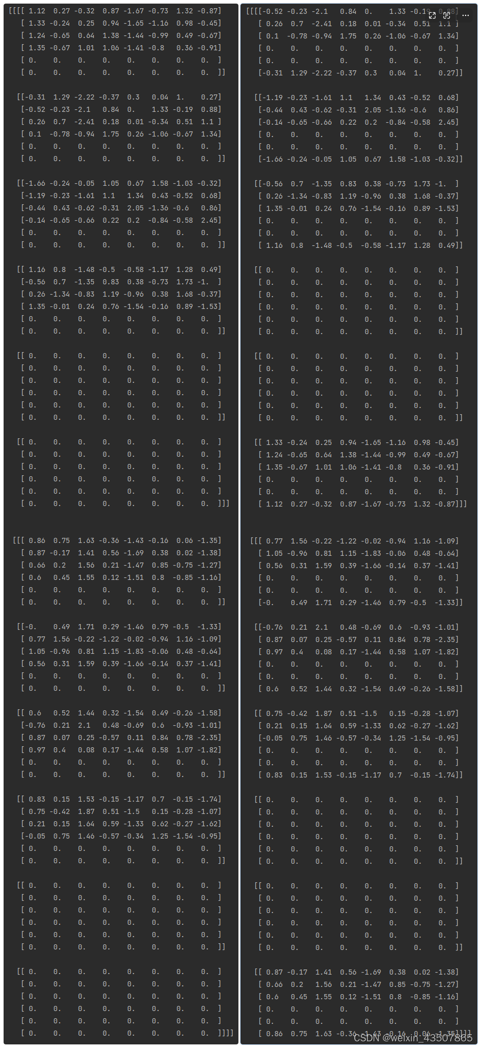
x = F.pad(x, (0, 0, pad_l, pad_r, pad_t, pad_b)) # (2, 6, 6, 8)x = F.pad(x, (0, 0, pad_l, pad_r, pad_t, pad_b))的结果如下:
3.2.1. WindowPartition
将feature map按照window_size划分成一个个没有重叠的window
def window_partition(x, window_size: int):
"""
将feature map按照window_size划分成一个个没有重叠的window
Args:
x: (B, H, W, C)
window_size (int): window size(M)
Returns:
windows: (num_windows*B, window_size, window_size, C)
"""
B, H, W, C = x.shape
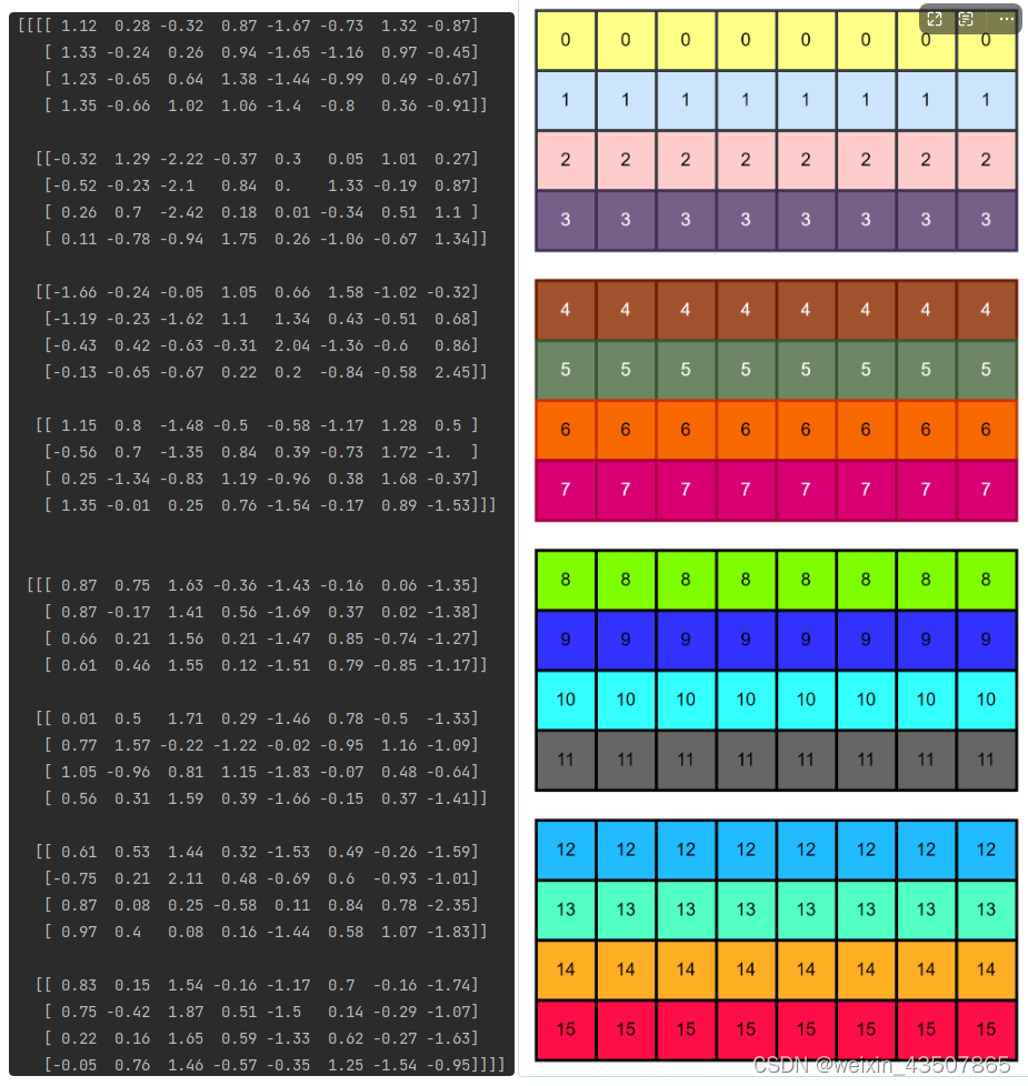
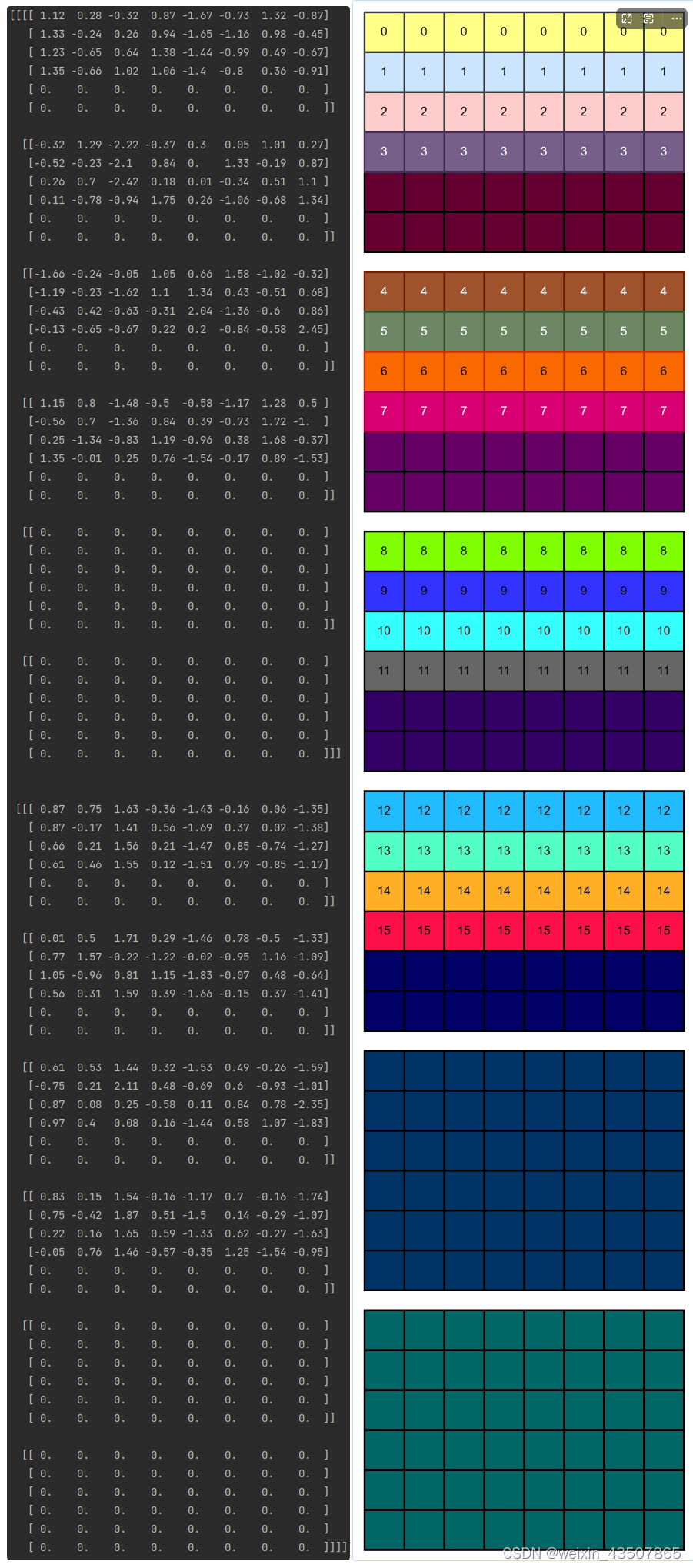
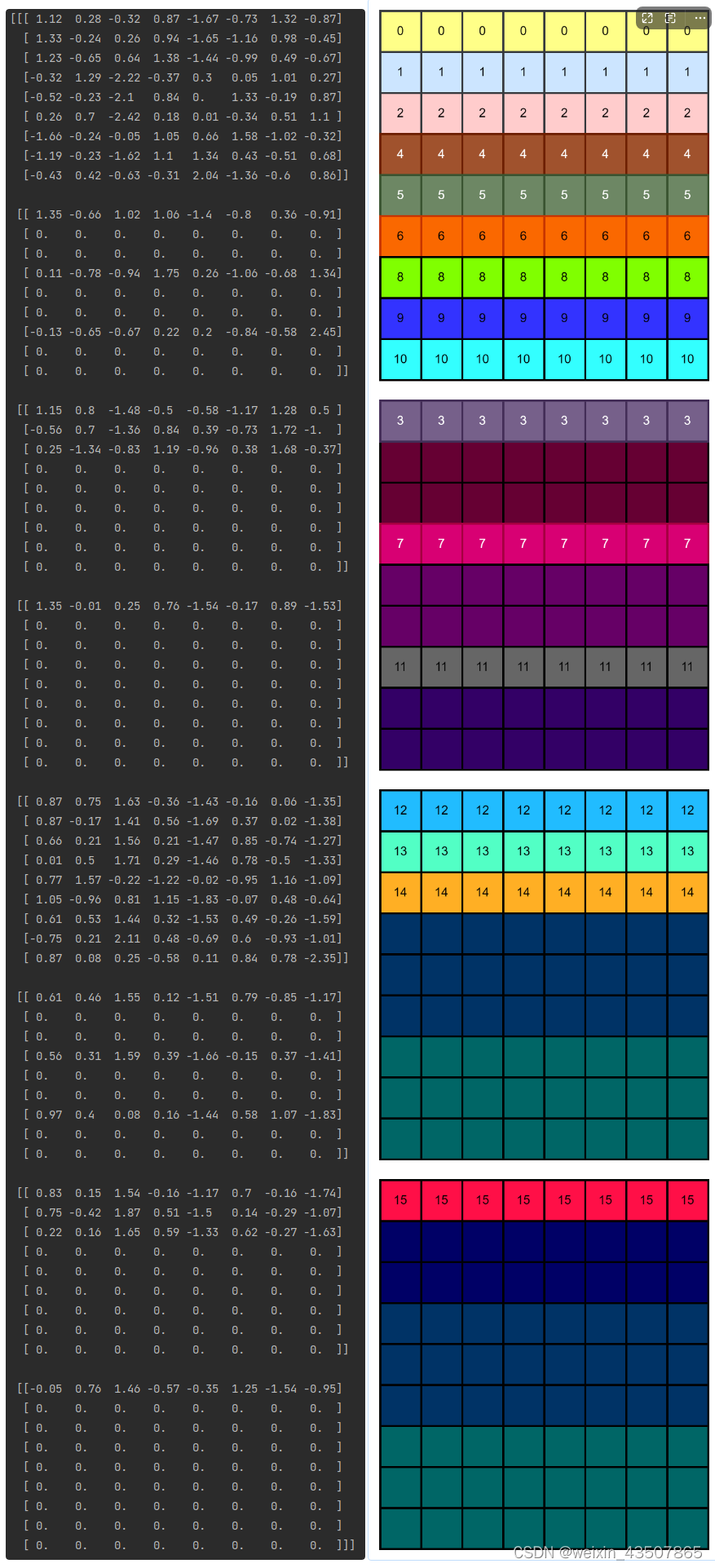
x = x.view(B, H // window_size, window_size, W // window_size, window_size, C) # (2,2,3,2,3,8)
# permute: [B, H//Mh, Mh, W//Mw, Mw, C] -> [B, H//Mh, W//Mh, Mw, Mw, C]
# view: [B, H//Mh, W//Mw, Mh, Mw, C] -> [B*num_windows, Mh, Mw, C]
windows = x.permute(0, 1, 3, 2, 4, 5).contiguous().view(-1, window_size, window_size, C) # (8,3,3,8)
return windowsx = x.view(B, H // window_size, window_size, W // window_size, window_size, C)的结果如下:
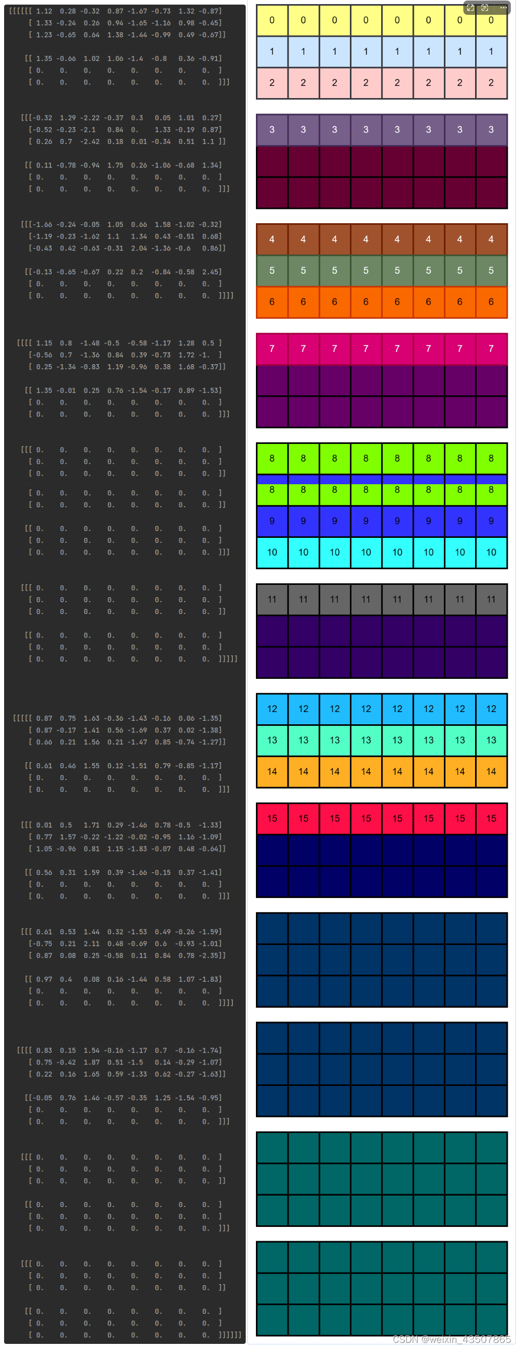
windows = x.permute(0, 1, 3, 2, 4, 5).contiguous().view(-1, window_size, window_size, C)的结果如下(8,3,3,8):
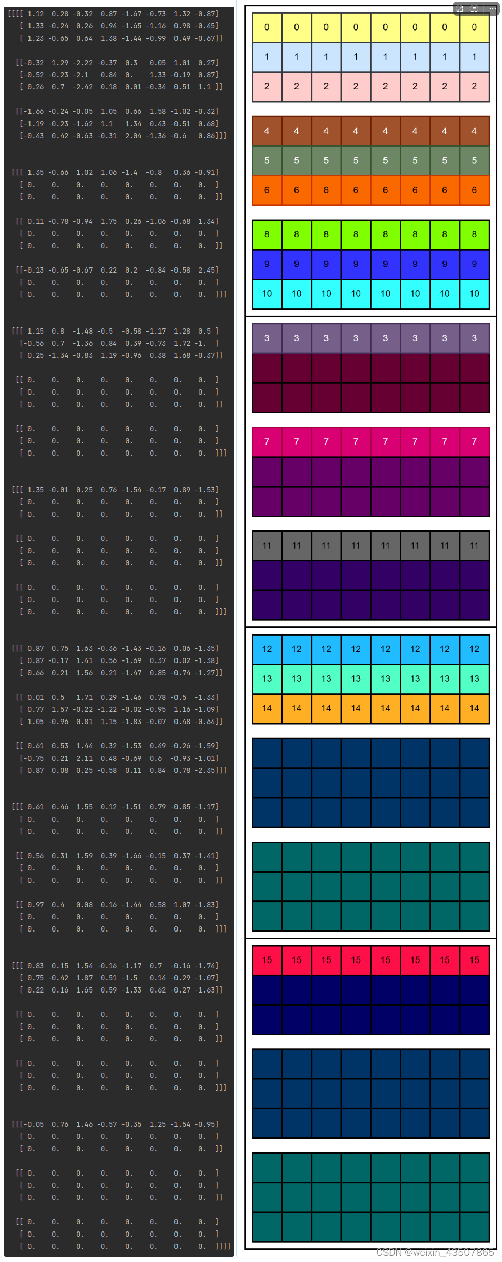
x_windows = x_windows.view(-1, self.window_size * self.window_size, C)的结果如下(8,9,8):
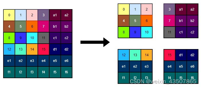
对于一张图片的特征图,划分出了 4 个 window,如下图所示:
3.2.2. q、k、v
qkv = self.qkv(x).reshape(B_, N, 3, self.num_heads, C // self.num_heads).permute(2, 0, 3, 1, 4)
w_q,w_k,w_v 的 shape 为(8, 24)
- qkv(): -> [batch_size*num_windows, Mh*Mw, 3 * total_embed_dim], [2*4, 3*3, 3*8]
- reshape: -> [batch_size*num_windows, Mh*Mw, 3, num_heads, embed_dim_per_head], [2*4, 3*3, 3, 2, 4]
- permute: -> [3, batch_size*num_windows, num_heads, Mh*Mw, embed_dim_per_head], [3, 2*4, 2, 3*3, 4]
q, k, v = qkv.unbind(0),将 q、k、v 拆分开
- q: ->[batch_size*num_windows, num_heads, Mh*Mw, embed_dim_per_head], [2*4, 2, 3*3, 4]
- k: ->[batch_size*num_windows, num_heads, Mh*Mw, embed_dim_per_head], [2*4, 2, 3*3, 4]
- v: ->[batch_size*num_windows, num_heads, Mh*Mw, embed_dim_per_head], [2*4, 2, 3*3, 4]
解释下上面 q(k 和 v 是一样的)的 shape, 一个 batch 中的每一张图片中的每一个 window 的每个 head 都有自己的 q、k、v 值。
3.2.3. 计算 attention
attention 的计算公式如下:
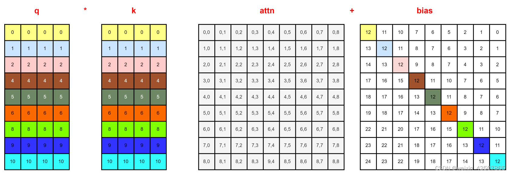
q = q * self.scale,即 Q / √d
attn = (q @ k.transpose(-2, -1)), @: multiply, q @ k.transpose(-2, -1)) 即。attn 的 shape 为(8, 2, 9, 9)
3.2.3.1. Relative Position Bias
swintransformer 使用了如下公式来计算最终的 attention 值,
上面公式中的 B 就是Relative Position Bias
3.2.3.2. relative position bias table
有一个relative position bias table,里面保存了每个相对位置的偏置参数,其大小为(2 * window_size[0] - 1) * (2 * window_size[1] - 1), num_heads)
self.relative_position_bias_table = nn.Parameter(torch.zeros((2 * window_size[0] - 1) * (2 * window_size[1] - 1), num_heads)),定义relative_position_bias_table 参数,初始值都为 0,shape 为(25, 2):
coords_h = torch.arange(self.window_size[0])
coords_w = torch.arange(self.window_size[1])
coords = torch.stack(torch.meshgrid([coords_h, coords_w], indexing="ij")) # [2, Mh, Mw]
coords_flatten = torch.flatten(coords, 1)
relative_coords = coords_flatten[:, :, None] - coords_flatten[:, None, :] # [2, Mh*Mw, Mh*Mw]
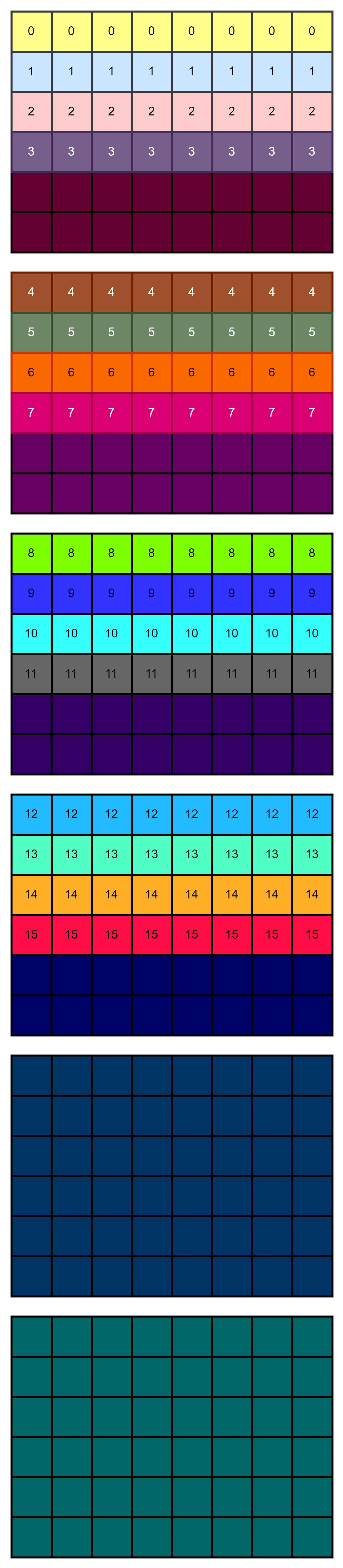
relative_coords = relative_coords.permute(1, 2, 0).contiguous() # [Mh*Mw, Mh*Mw, 2]relative_coords 的结果如下:
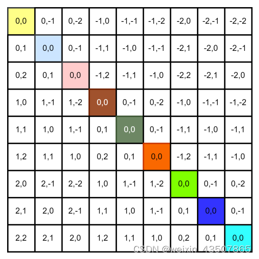
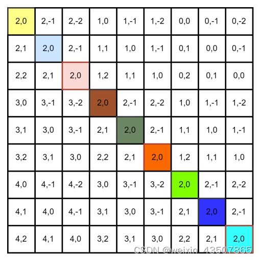
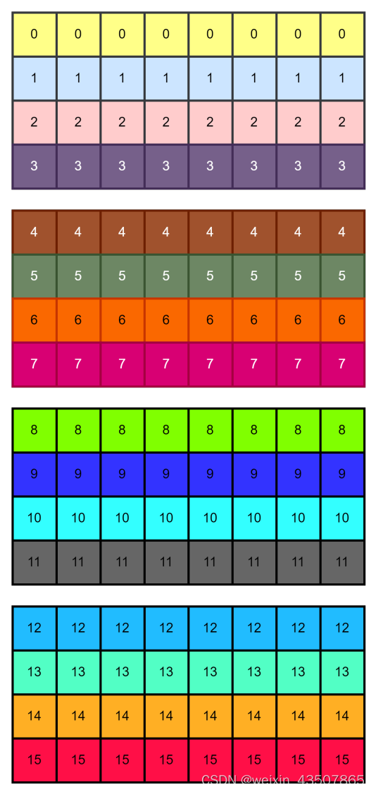
relative_coords[:, :, 0] += self.window_size[0] - 1 , 每个位置的横坐标+2,结果如下:
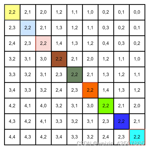
relative_coords[:, :, 1] += self.window_size[1] - 1 ,每个位置的纵坐标+2,结果如下:
relative_coords[:, :, 0] *= 2 * self.window_size[1] - 1 ,每个位置的横坐标 * 5,结果如下:

relative_position_index = relative_coords.sum(-1)的结果如下:
根据relative_position_index 从relative_position_bias_table 中查找偏置值
relative_position_bias = self.relative_position_bias_table[self.relative_position_index.view(-1)].view(self.window_size[0] * self.window_size[1], self.window_size[0] * self.window_size[1], -1),shape 为(9, 9, 2)
relative_position_bias = relative_position_bias.permute(2, 0, 1).contiguous(),shape 为(2, 9, 9), 表示
attn = attn + relative_position_bias.unsqueeze(0), (8, 2, 9, 9) + (2, 9, 9) = (8, 2, 9, 9)
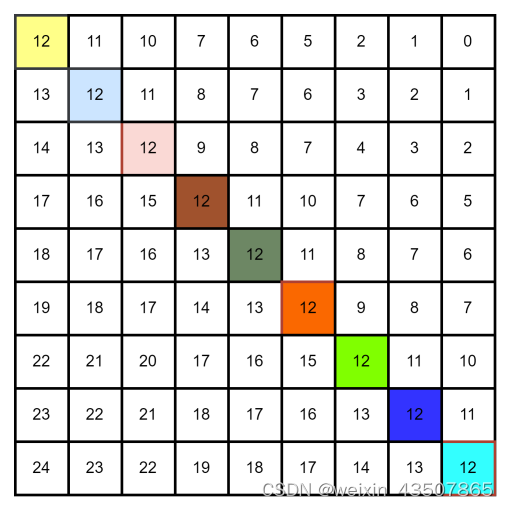
以一个 window 举例,如下图所示:
attn = self.softmax(attn),即公式
中的 softmax 函数。
x = (attn @ v).transpose(1, 2).reshape(B_, N, C),其中attn @ v 即为公式中的最后一个部分。reshape 之后的 shape 为(8, 9, 8)。
attn_windows = self.attn(x_windows, mask=attn_mask), 到这里 attn 就计算完了。
attn_windows = attn_windows.view(-1, self.window_size, self.window_size, C),shape 为(8, 3, 3, 8)
shifted_x = window_reverse(attn_windows, self.window_size, Hp, Wp),将一个个 window 还原成 feature map。shape 为(2, 6, 6, 8),其中 2 表示 batch_size;8 表示特征维度,又还原成下图的样子了(针对一张图片):
从上图看出,还有之前 pad 的数据,因此需要把它移除掉。x = x[:, :H, :W, :].contiguous(),shape 为(2, 4, 4, 8)
再对维度进行整合,x = x.view(B, H * W, C),shape 为(2, 16, 8)
3.3. W-MSA 中的第二个 LN 层 + MLP
x = shortcut + self.drop_path(x)
x = x + self.drop_path(self.mlp(self.norm2(x)))
3.4. SW-MSA 中第一个 LN 层
进入到 SW-MSA 部分,先还是有一个 LN 层,代码和之前的代码都是一样的。
3.5. SW-MSA
3.5.1. 特征图滑动
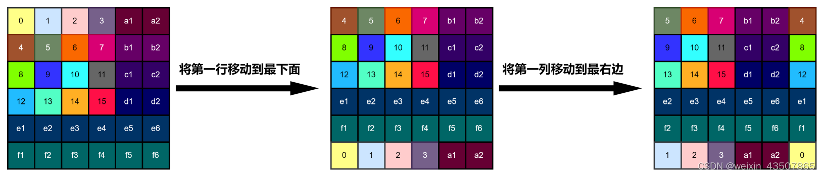
shifted_x = torch.roll(x, shifts=(-self.shift_size, -self.shift_size), dims=(1, 2)),
x 如左图所示,shifted_x 如右图所示:
用特征图表示如下:
3.5.2. WindowPartition
同 W-MSA 部分的代码一样,这里就不再重复了。得到 4 个 window 的特征图,如下图所示:

3.5.3. attention mask
先说一下为什么需要 attention mask,在 SW-MSA 中,需要对特征图进行滑动,如下图所示:
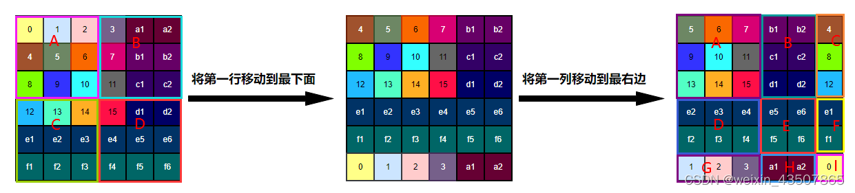
说明:在我的代码中,生成的特征图是 4*4 的,而 window_size 为 3,因此需要对特征图进行扩充,以适应窗口大小。上图用字母标注的区域都是扩充的部分;
对于滑动之后的特征图,如果还是像 W-MSA 中直接对每个 3*3 的窗口计算 attention 值的话,就会有问题。
滑动后新生成的 4 的 window,对于第一个 window,可以直接计算 attention 值,这是没有问题的。但是对于第 2、3、4 个窗口,就不能直接计算 attention 值了,信息会乱窜。
上图所示,需要单独对每个子区域计算 attention 值,相当于总共要计算 9 个区域的 attention 值。但是在 W-MSA 中,只计算了 4 个区域的 attention 值,为了保证计算量一样,源码中引入了 attention mask。其作用是还是计算 4 个区域的 attention 值,但是对于第 2、3、4 个窗口,每个子区域单独计算 attention 值。
attention mask 的生成过程如下:
img_mask(1, 6, 6, 1)
Hp = int(np.ceil(H / self.window_size)) * self.window_size	# window_size=3  Hp=6
Wp = int(np.ceil(W / self.window_size)) * self.window_size	# Wp = 6
# 拥有和feature map一样的通道排列顺序,方便后续window_partition
img_mask = torch.zeros((1, Hp, Wp, 1), device=x.device)
h_slices = (slice(0, -self.window_size),
            slice(-self.window_size, -self.shift_size),
            slice(-self.shift_size, None))
w_slices = (slice(0, -self.window_size),
            slice(-self.window_size, -self.shift_size),
            slice(-self.shift_size, None))
cnt = 0
for h in h_slices:
    for w in w_slices:
        img_mask[:, h, w, :] = cnt
        cnt += 1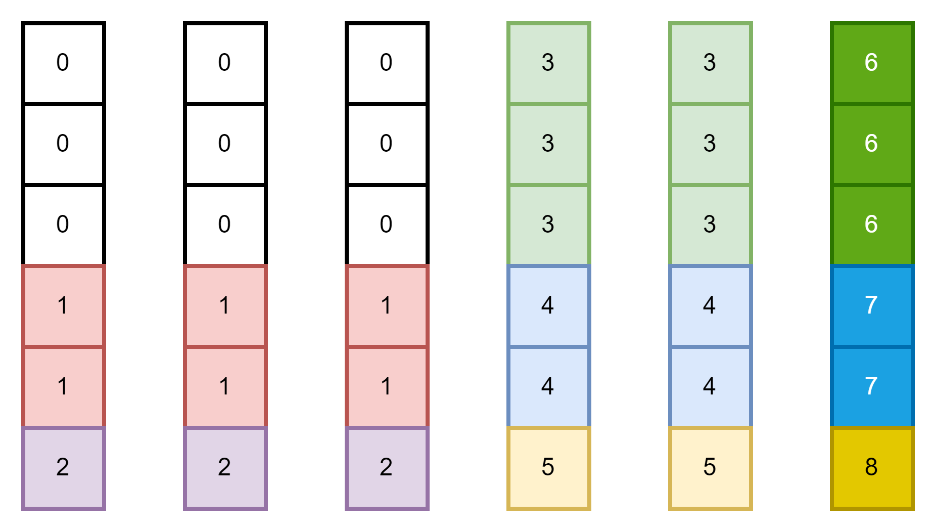
mask_window(4, 9)
mask_windows = window_partition(img_mask, self.window_size)  # [nW, Mh, Mw, 1]
mask_windows = mask_windows.view(-1, self.window_size * self.window_size)  # [nW, Mh*Mw]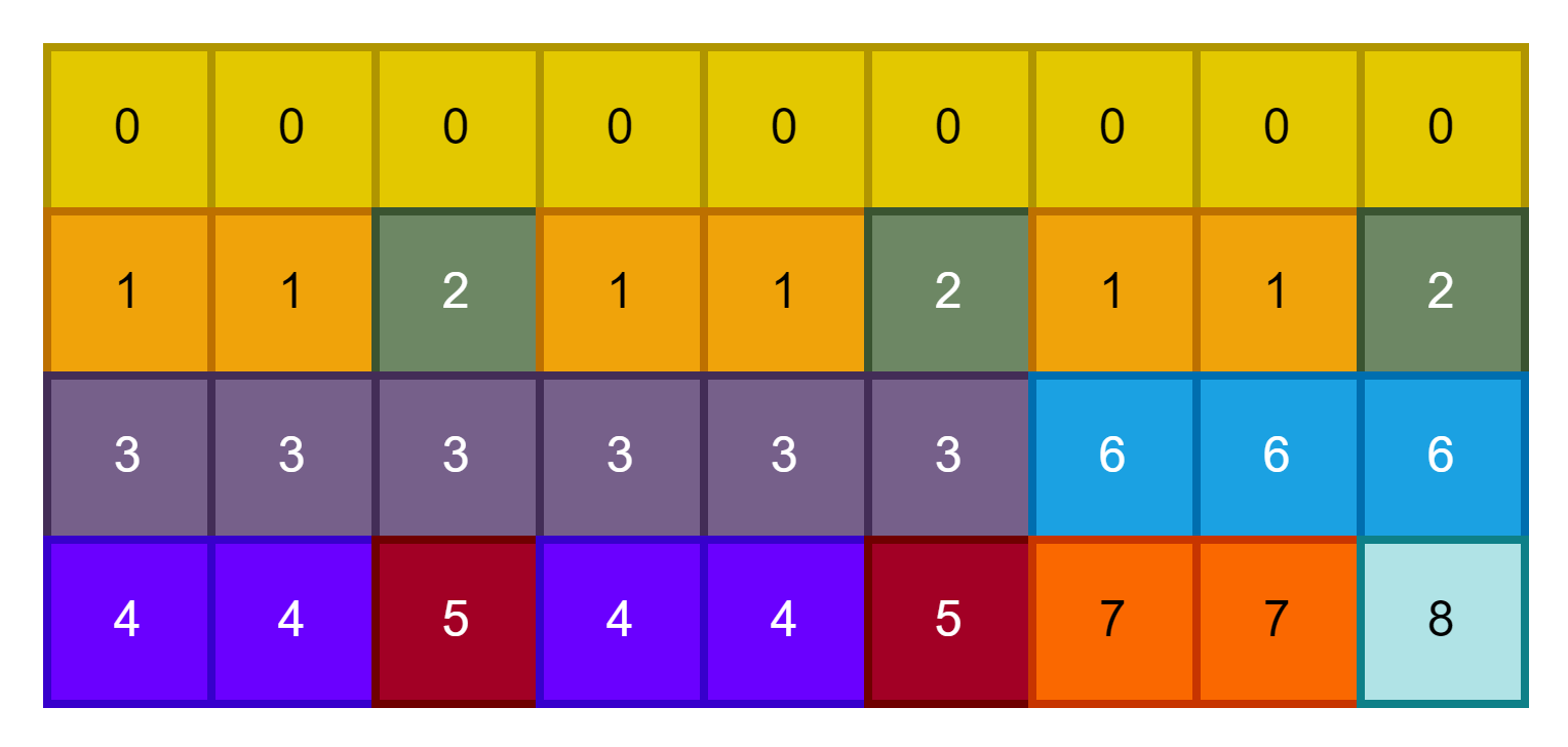
attn_mask(4, 9, 9)
attn_mask = mask_windows.unsqueeze(1) - mask_windows.unsqueeze(2)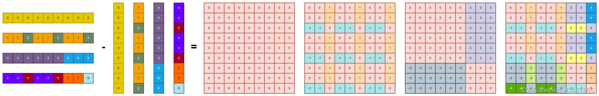
attn_mask = attn_mask.masked_fill(attn_mask != 0, float(-100.0)).masked_fill(attn_mask == 0, float(0.0))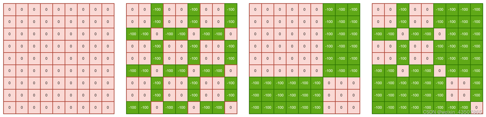
3.5.4. 计算 attention
每个 window 的 q 和 k 矩阵进行计算,得到 9*9 的 attention 矩阵
attn = (q @ k.transpose(-2, -1))然后加上相对位置的偏移值
relative_position_bias = self.relative_position_bias_table[self.relative_position_index.view(-1)].view(
    self.window_size[0] * self.window_size[1], self.window_size[0] * self.window_size[1], -1)
relative_position_bias = relative_position_bias.permute(2, 0, 1).contiguous()  # [nH, Mh*Mw, Mh*Mw]
attn = attn + relative_position_bias.unsqueeze(0)
然后加上 attention mask
if mask is not None:
    # mask: [nW, Mh*Mw, Mh*Mw]
    nW = mask.shape[0]  # num_windows
    # attn.view: [batch_size, num_windows, num_heads, Mh*Mw, Mh*Mw],[2, 4, 2, 9, 9]
    # mask.unsqueeze: [1, nW, 1, Mh*Mw, Mh*Mw], [1, 4, 1, 9, 9]
    attn = attn.view(B_ // nW, nW, self.num_heads, N, N) + mask.unsqueeze(1).unsqueeze(0)
    attn = attn.view(-1, self.num_heads, N, N)
    attn = self.softmax(attn)
如下图所示:
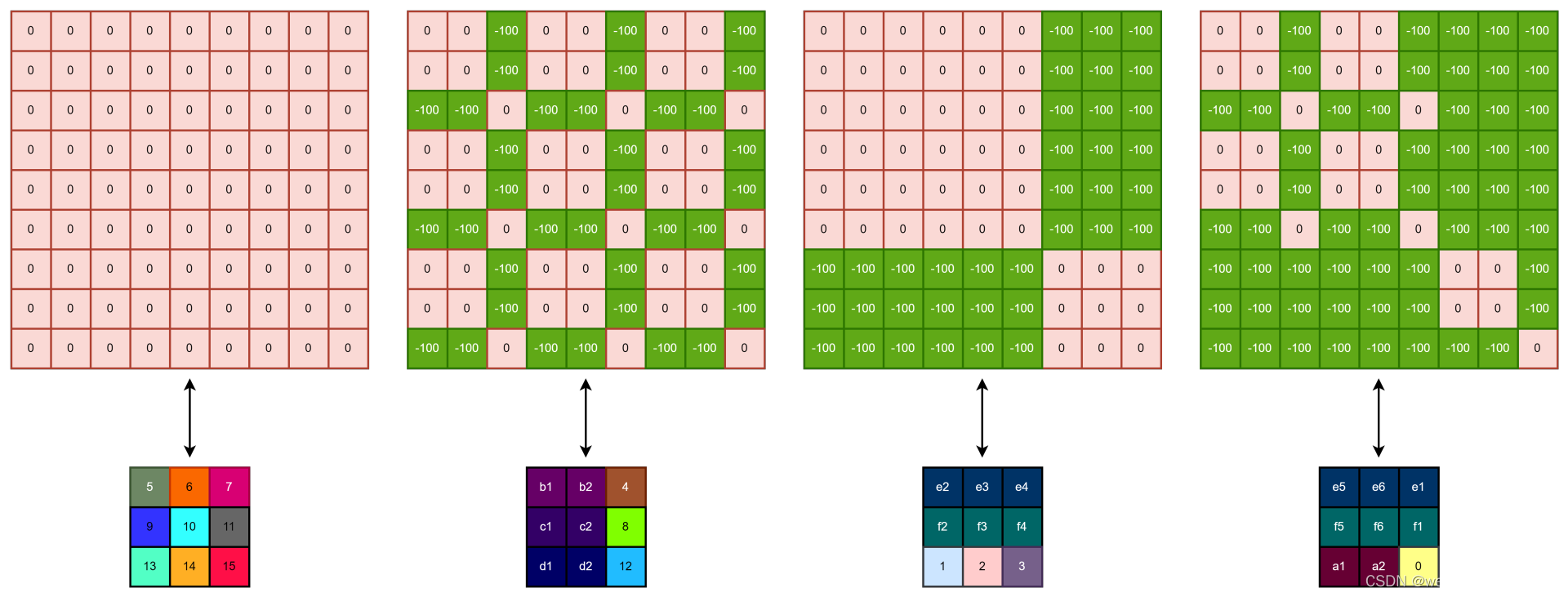
即,每个窗口的子区域单独计算 attention 值。
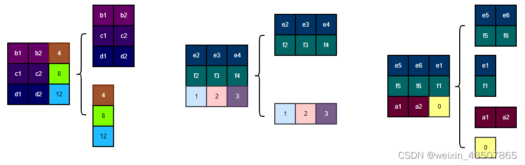
举个例子:上图中的第二个 window,b1 的 q 只需要同 b1、b2、c1、c2、d1、d2 的 k 计算 attention 值,即 q_b1*k_b1, q_b1*k_b2,q_b1*k_4,q_b1*k_c1,q_b1*k_c2,q_b1*k_8,q_b1*k_d1,q_b1*k_d2,q_b1*k_12,红色的部分就是上图中第一行的三个-100 值的位置,-100 的位置在经过 softmax 之后就会变成 0,相当于没有计算当前位置的 attention 值。
3.6. SW-MSA 中的第二个 LN 层 + MLP
x = shortcut + self.drop_path(x)
x = x + self.drop_path(self.mlp(self.norm2(x)))
4. PatchMerging
def forward(self, x, H, W):
    """
    x: B, H*W, C
    """
    B, L, C = x.shape
    assert L == H * W, "input feature has wrong size"

    x = x.view(B, H, W, C)

    # padding
    # 如果输入feature map的H,W不是2的整数倍,需要进行padding
    pad_input = (H % 2 == 1) or (W % 2 == 1)
    if pad_input:
        # to pad the last 3 dimensions, starting from the last dimension and moving forward.
        # (C_front, C_back, W_left, W_right, H_top, H_bottom)
        # 注意这里的Tensor通道是[B, H, W, C],所以会和官方文档有些不同
        x = F.pad(x, (0, 0, 0, W % 2, 0, H % 2))

    x0 = x[:, 0::2, 0::2, :]  # [B, H/2, W/2, C]
    x1 = x[:, 1::2, 0::2, :]  # [B, H/2, W/2, C]
    x2 = x[:, 0::2, 1::2, :]  # [B, H/2, W/2, C]
    x3 = x[:, 1::2, 1::2, :]  # [B, H/2, W/2, C]
    x = torch.cat([x0, x1, x2, x3], -1)  # [B, H/2, W/2, 4*C]
    x = x.view(B, -1, 4 * C)  # [B, H/2*W/2, 4*C]

    x = self.norm(x)
    x = self.reduction(x)  # [B, H/2*W/2, 2*C]

    return x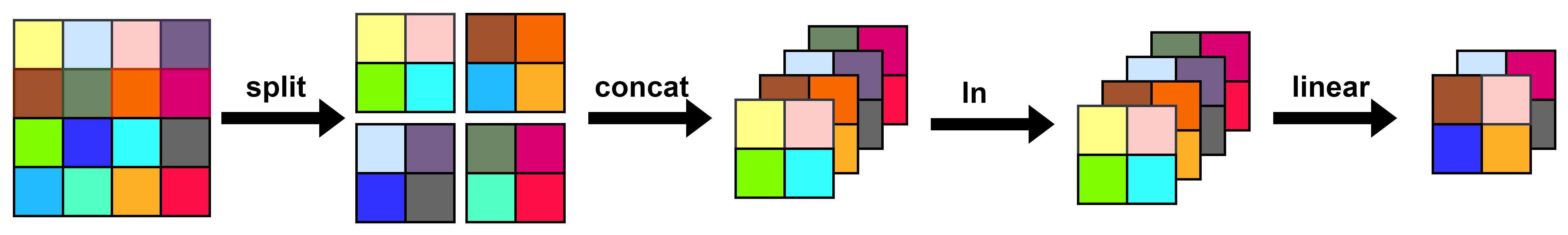
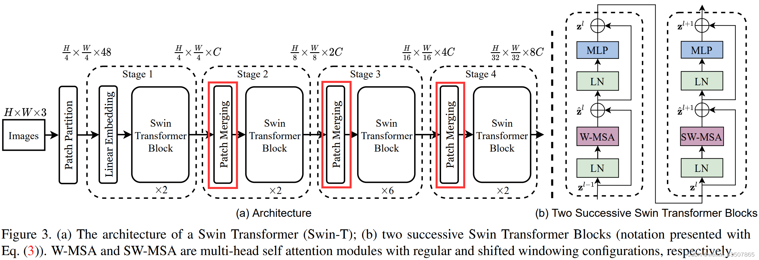
将上一次的特征图缩小为原来的一半,特征维度增加为原来的 2 倍。


 1887
1887

 被折叠的 条评论
为什么被折叠?
被折叠的 条评论
为什么被折叠?
 到【灌水乐园】发言


