Faster_RCNN的读取和数据处理

最近开始学习目标检测faster rcnn，首先看了很多博客讲解原理，然后从github上下载tensorflow版本的代码，代码太长看了好几天没明白，后来看到了chenyuntc的 simple-faster-rcnn-pytorch，还有作者写这份代码的心得，让我感觉很佩服，自认为目前阶段不能手写如此复杂的代码。作者是从tf版本的改为pytorch版的，我在学习的过程中也查阅了很多其他人写的讲解代码的博客，得到了很大的帮助，所以也打算把自己一些粗浅的理解记录下来，一是记录下自己的菜鸟学习之路，方便自己过后查阅，二来可以回馈网络。目前编程能力有限，且是第一次写博客，中间可能会有一些错误。

第一步 跑通代码
第二步 数据预处理
第三步 模型准备
第四步 训练代码

第一步 跑通代码

作者的README.MD部分讲解的很清楚了，一步一步安装PyTorch，cupy，然后运行pip install -r requirements.txt安装各种包。我用的是自己的台式机，1070GPU，python3.6，windows环境。安装PyTorch>=0.4时上官网根据自己的环境去找对应的pip指令安装时可能下载速度巨慢，我是直接下载了torch-0.4.1-cp36-cp36m-win_amd64.whl，运行pip install torch-0.4.1-cp36-cp36m-win_amd64.whl安装的，这里我将文件放到云盘上有需要自取https://pan.baidu.com/s/1pqSpeTFH3ooh7q1M3vrtfQ,提取码：hda0。cupy安装时出错了，提示我需要安装VS，注意最好安装vs2015以上版本。接下来是build cython code nms_gpu_post，这里我一直报错，后来发现是可选择运行的，我就直接跳过了，不过作者说最好运行这一步。然后是下载预训练模型，数据集，解压数据集操作。需要将util/config.py中voc_data_dir改为自己的路径，通过执行python misc/convert_caffe_pretrain.py，下载caffe_pretrain预训练模型，我是直接将caffe_pretrain改为True了，如果设置false则直接会下载pytorch版本的预训练模型。然后在终端下运行python -m visdom.server，弹出一个网址打开。visdom是类似tensorflow中的tensorboard的工具，可以可视化训练过程中的各种曲线或者图，然后运行python train. py train --env=‘fasterrcnn-caffe’ --plot-every=100 --caffe-pretrain，就开始了训练过程，可以看到网页中出现了5个loss曲线图，还有一个标签图和预测图。类似下面这样的

第二步 数据预处理

1.data/dataset.py文件（主代码中调用的其他重要函数会在后面按顺序讲解）

#去正则化,img维度为[[B,G,R],H,W],因为caffe预训练模型输入为BGR 0-255图片，pytorch预训练模型采用RGB 0-1图片
def inverse_normalize(img):
    if opt.caffe_pretrain:   #如果采用caffe预训练模型，则返回 img[::-1, :, :]，如果不采用，则返回(img * 0.225 + 0.45).clip(min=0, max=1) * 255 
        img = img + (np.array([122.7717, 115.9465, 102.9801]).reshape(3, 1, 1))   #[122.7717, 115.9465, 102.9801]reshape为[3,1,1]与img维度相同就可以相加了，caffe_normalize之前有减均值预处理，现在还原回去。
        return img[::-1, :, :]     #将BGR转换为RGB图片（python [::-1]为逆序输出）
    return (img * 0.225 + 0.45).clip(min=0, max=1) * 255    #pytorch_normalze中标准化为减均值除以标准差，现在乘以标准差加上均值还原回去，转换为0-255

#采用pytorch预训练模型对图片预处理，函数输入的img为0-1

def pytorch_normalze(img):
    normalize = tvtsf.Normalize(mean=[0.485, 0.456, 0.406], std=[0.229, 0.224, 0.225])  #transforms.Normalize使用如下公式进行归一化channel=（channel-mean）/std,转换为[-1,1]
    img = normalize(t.from_numpy(img))     #(ndarray) → Tensor
    return img.numpy()
    
 #采用caffe预训练模型时对输入图像进行标准化，函数输入的img为0-1

 def caffe_normalize(img):
    img = img[[2, 1, 0], :, :]  # RGB-BGR
    img = img * 255
    mean = np.array([122.7717, 115.9465, 102.9801]).reshape(3, 1, 1) #转换为与img维度相同
    img = (img - mean).astype(np.float32, copy=True)   #减均值操作
    return img
    
 #函数输入的img为0-255

def preprocess(img, min_size=600, max_size=1000): #按照论文长边不超1000，短边不超600。按此比例缩放
    C, H, W = img.shape
    scale1 = min_size / min(H, W)
    scale2 = max_size / max(H, W)
    scale = min(scale1, scale2)    #选小的比例，这样长和宽都能放缩到规定的尺寸
    img = img / 255  #转换为0-1
    img = sktsf.resize(img, (C, H * scale, W * scale), mode='reflect',anti_aliasing=False) #resize到（H * scale, W * scale）大小，anti_aliasing为是否采用高斯滤波
#调用pytorch_normalze或者caffe_normalze对图像进行正则化
    if opt.caffe_pretrain:
        normalize = caffe_normalize
    else:
        normalize = pytorch_normalze
    return normalize(img)
 
class Transform(object):
    def __init__(self, min_size=600, max_size=1000):
        self.min_size = min_size
        self.max_size = max_size
    def __call__(self, in_data):
        img, bbox, label = in_data
        _, H, W = img.shape
        img = preprocess(img, self.min_size, self.max_size)  #图像等比例缩放
        _, o_H, o_W = img.shape 
        scale = o_H / H   #得出缩放比因子
        bbox = util.resize_bbox(bbox, (H, W), (o_H, o_W))  #bbox按照与原图等比例缩放

        # horizontally flip
        img, params = util.random_flip(
            img, x_random=True, return_param=True) #将图片进行随机水平翻转，没有进行垂直翻转
        bbox = util.flip_bbox(
            bbox, (o_H, o_W), x_flip=params['x_flip']) #同样地将bbox进行与对应图片同样的水平翻转
        return img, bbox, label, scale 
        
class Dataset:      #训练集样本的生成
    def __init__(self, opt):
        self.opt = opt
        self.db = VOCBboxDataset(opt.voc_data_dir)   #实例化类
        self.tsf = Transform(opt.min_size, opt.max_size) ##实例化类
    def __getitem__(self, idx):   #__ xxx__运行Dataset类时自动运行
        ori_img, bbox, label, difficult = self.db.get_example(idx) #调用VOCBboxDataset中的get_example（）从数据集存储路径中将img, bbox, label, difficult 一个个的获取出来
        img, bbox, label, scale = self.tsf((ori_img, bbox, label)) #调用前面的Transform函数将图片,label进行最小值最大值放缩归一化，重新调整bboxes的大小，然后随机反转，最后将数据集返回
        return img.copy(), bbox.copy(), label.copy(), scale
    def __len__(self):
        return len(self.db)  

class TestDataset:   #测试集样本的生成
    def __init__(self, opt, split='test', use_difficult=True):
        self.opt = opt
        self.db = VOCBboxDataset(opt.voc_data_dir, split=split, use_difficult=use_difficult)  #此处设置了use_difficult,

    def __getitem__(self, idx):
        ori_img, bbox, label, difficult = self.db.get_example(idx)
        img = preprocess(ori_img)
        return img, ori_img.shape[1:], bbox, label, difficult

    def __len__(self):
        return len(self.db)

下面是data/util.py文件

def resize_bbox(bbox, in_size, out_size):
    bbox = bbox.copy()
    y_scale = float(out_size[0]) / in_size[0]
    x_scale = float(out_size[1]) / in_size[1]  #获得与原图同样的缩放比
    bbox[:, 0] = y_scale * bbox[:, 0]
    bbox[:, 2] = y_scale * bbox[:, 2]
    bbox[:, 1] = x_scale * bbox[:, 1]
    bbox[:, 3] = x_scale * bbox[:, 3]  #按与原图同等比例缩放bbox
    return bbox
    
 def random_flip(img, y_random=False, x_random=False,
                return_param=False, copy=False):
    y_flip, x_flip = False, False
    if y_random:   #False
        y_flip = random.choice([True, False])
    if x_random:   #True
        x_flip = random.choice([True, False])  #随机选择图片是否进行水平翻转

    if y_flip:
        img = img[:, ::-1, :]
    if x_flip:
        img = img[:, :, ::-1]   #python [::-1]为逆序输出，这里指水平翻转
    if copy:
        img = img.copy()
    if return_param:   #True
        return img, {'y_flip': y_flip, 'x_flip': x_flip}  #返回img和x_flip(为了让bbox有同样的水平翻转操作)
    else:
        return img

 def flip_bbox(bbox, size, y_flip=False, x_flip=False):  
    H, W = size  #缩放后图片的size
    bbox = bbox.copy()
    if y_flip:              #没有进行垂直翻转
        y_max = H - bbox[:, 0]
        y_min = H - bbox[:, 2]
        bbox[:, 0] = y_min
        bbox[:, 2] = y_max
    if x_flip:
        x_max = W - bbox[:, 1]  
        x_min = W - bbox[:, 3] #计算水平翻转后左下角和右上角的坐标
        bbox[:, 1] = x_min
        bbox[:, 3] = x_max
    return bbox

下面是data/voc_dataset.py文件

VOCBboxDataset:
    def __init__(self, data_dir, split='trainval',
                 use_difficult=False, return_difficult=False,
                 ):
        id_list_file = os.path.join(
            data_dir, 'ImageSets/Main/{0}.txt'.format(split))  # id_list_file为split.txt，split为'trainval'或者'test'
        self.ids = [id_.strip() for id_ in open(id_list_file)] #id_为每个样本文件名
        self.data_dir = data_dir #写到/VOC2007/的路径
        self.use_difficult = use_difficult 
        self.return_difficult = return_difficult 
        self.label_names = VOC_BBOX_LABEL_NAMES   #20类

    def __len__(self):
        return len(self.ids)  #trainval.txt有5011个，test.txt有210个
    def get_example(self, i):
        id_ = self.ids[i]
        anno = ET.parse(
            os.path.join(self.data_dir, 'Annotations', id_ + '.xml'))  #读入 xml标签文件
        bbox = list()
        label = list()
        difficult = list()
        #解析xml文件
        for obj in anno.findall('object'):
            if not self.use_difficult and int(obj.find('difficult').text) == 1:  #标为difficult的目标在测试评估中一般会被忽略
                continue   #xml文件中包含object name和difficult(0或者1,0代表容易检测)
            difficult.append(int(obj.find('difficult').text)) 
            bndbox_anno = obj.find('bndbox')  #bndbox（xmin,ymin,xmax,ymax),表示框左下角和右上角坐标
            bbox.append([
                int(bndbox_anno.find(tag).text) - 1  
                for tag in ('ymin', 'xmin', 'ymax', 'xmax')]) #让坐标基于（0,0）
            name = obj.find('name').text.lower().strip()  #框中object name
            label.append(VOC_BBOX_LABEL_NAMES.index(name))  
        bbox = np.stack(bbox).astype(np.float32)   #所有object的bbox坐标存在列表里
        label = np.stack(label).astype(np.int32)     #所有object的label存在列表里
        # When `use_difficult==False`, all elements in `difficult` are False.
        difficult = np.array(difficult, dtype=np.bool).astype(np.uint8)  # PyTorch 不支持 np.bool，所以这里转换为uint8
        img_file = os.path.join(self.data_dir, 'JPEGImages', id_ + '.jpg') #根据图片编号在/JPEGImages/取图片
        img = read_image(img_file, color=True)    #如果color=True，则转换为RGB图
        return img, bbox, label, difficult
    __getitem__ = get_example  #一般如果想使用索引访问元素时，就可以在类中定义这个方法（__getitem__(self, key) )

第三步 模型准备

下面看的是model/util/文件夹，主要是进行一些配置文件
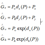
首先看的是bbox_tools.py文件,其中涉及RCNN中提出的边框回归公式，G^表示近似目标边框，P表示proposal边框,回归学习（我觉得可以参考下这个博客辅助理解）就是偏移量dx,dy,dh,dw这四个变换，让CNN提取的特征乘以w的转置

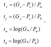
真正目标边框与proposal之间的偏移即为下面的tx，ty，tw，th

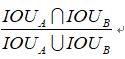
交并比公式：

另外NMS处理可以参考这篇博客

def loc2bbox(src_bbox, loc): #已知源bbox 和位置偏差dx，dy，dh，dw，求目标框G
    if src_bbox.shape[0] == 0:
        return xp.zeros((0, 4), dtype=loc.dtype)        #src_bbox：（R，4），R为bbox个数，4为左下角和右上角四个坐标(这里有误，按照标准坐标系中y轴向下，应该为左上和右下角坐标)
    src_bbox = src_bbox.astype(src_bbox.dtype, copy=False) 
    src_height = src_bbox[:, 2] - src_bbox[:, 0]      #ymax-ymin
    src_width = src_bbox[:, 3] - src_bbox[:, 1]     #xmax-xmin
    src_ctr_y = src_bbox[:, 0] + 0.5 * src_height    y0+0.5h
    src_ctr_x = src_bbox[:, 1] + 0.5 * src_width   #x0+0.5w,计算出中心点坐标
#src_height为Ph,src_width为Pw，src_ctr_y为Py，src_ctr_x为Px
    dy = loc[:, 0::4]      #python [start:stop:step] 
    dx = loc[:, 1::4]
    dh = loc[:, 2::4]
    dw = loc[:, 3::4]
RCNN中提出的边框回归：寻找原始proposal与近似目标框G之间的映射关系，公式在上面
    ctr_y = dy * src_height[:, xp.newaxis] + src_ctr_y[:, xp.newaxis]  #ctr_y为Gy
    ctr_x = dx * src_width[:, xp.newaxis] + src_ctr_x[:, xp.newaxis] # ctr_x为Gx
    h = xp.exp(dh) * src_height[:, xp.newaxis] #h为Gh
    w = xp.exp(dw) * src_width[:, xp.newaxis] #w为Gw
#上面四行得到了回归后的目标框（Gx,Gy,Gh,Gw）
    dst_bbox = xp.zeros(loc.shape, dtype=loc.dtype)  #loc.shape：（R，4），同src_bbox
    dst_bbox[:, 0::4] = ctr_y - 0.5 * h
    dst_bbox[:, 1::4] = ctr_x - 0.5 * w
    dst_bbox[:, 2::4] = ctr_y + 0.5 * h
    dst_bbox[:, 3::4] = ctr_x + 0.5 * w   #由中心点转换为左上角和右下角坐标
    return dst_bbox
    
def bbox2loc(src_bbox, dst_bbox): #已知源框和目标框求出其位置偏差
    height = src_bbox[:, 2] - src_bbox[:, 0]
    width = src_bbox[:, 3] - src_bbox[:, 1]
    ctr_y = src_bbox[:, 0] + 0.5 * height
    ctr_x = src_bbox[:, 1] + 0.5 * width #计算出源框中心点坐标

    base_height = dst_bbox[:, 2] - dst_bbox[:, 0]
    base_width = dst_bbox[:, 3] - dst_bbox[:, 1]
    base_ctr_y = dst_bbox[:, 0] + 0.5 * base_height
    base_ctr_x = dst_bbox[:, 1] + 0.5 * base_width ##计算出目标框中心点坐标

    eps = xp.finfo(height.dtype).eps  #求出最小的正数
    height = xp.maximum(height, eps) 
    width = xp.maximum(width, eps)  #将height,width与其比较保证全部是非负

    dy = (base_ctr_y - ctr_y) / height
    dx = (base_ctr_x - ctr_x) / width
    dh = xp.log(base_height / height)
    dw = xp.log(base_width / width)  #根据上面的公式二计算dx，dy，dh，dw

    loc = xp.vstack((dy, dx, dh, dw)).transpose()    #np.vstack按照行的顺序把数组给堆叠起来
    return loc

def bbox_iou(bbox_a, bbox_b):  #求两个bbox的相交的交并比
    if bbox_a.shape[1] != 4 or bbox_b.shape[1] != 4:
        raise IndexError  #确保bbox第二维为bbox的四个坐标（ymin，xmin，ymax，xmax）
    tl = xp.maximum(bbox_a[:, None, :2], bbox_b[:, :2])  #tl为交叉部分框左上角坐标最大值，为了利用numpy的广播性质，bbox_a[:, None, :2]的shape是(N,1,2)，bbox_b[:, :2]shape是(K,2),由numpy的广播性质，两个数组shape都变成(N,K,2)，也就是对a里每个bbox都分别和b里的每个bbox求左上角点坐标最大值
    br = xp.minimum(bbox_a[:, None, 2:], bbox_b[:, 2:]) #br为交叉部分框右下角坐标最小值
    area_i = xp.prod(br - tl, axis=2) * (tl < br).all(axis=2) #所有坐标轴上tl<br时，返回数组元素的乘积(y1max-yimin)X(x1max-x1min)，bboxa与bboxb相交区域的面积
    area_a = xp.prod(bbox_a[:, 2:] - bbox_a[:, :2], axis=1)  #计算bboxa的面积
    area_b = xp.prod(bbox_b[:, 2:] - bbox_b[:, :2], axis=1) #计算bboxb的面积
    return area_i / (area_a[:, None] + area_b - area_i) #计算IOU

def generate_anchor_base(base_size=16, ratios=[0.5, 1, 2], #
                         anchor_scales=[8, 16, 32]):   #对特征图features以基准长度为16、选择合适的ratios和scales取基准锚点anchor_base。（选择长度为16的原因是图片大小为600*800左右，基准长度16对应的原图区域是256*256，考虑放缩后的大小有128*128，512*512比较合适）
#根据基准点生成9个基本的anchor的功能，ratios=[0.5,1,2],anchor_scales=[8,16,32]是长宽比和缩放比例,anchor_scales也就是在base_size的基础上再增加的量，本代码中对应着三种面积的大小(16*8)^2 ,(16*16)^2  (16*32)^2  也就是128,256,512的平方大小
    py = base_size / 2.
    px = base_size / 2.   

    anchor_base = np.zeros((len(ratios) * len(anchor_scales), 4),     
                           dtype=np.float32)  #（9，4），注意：这里只是以特征图的左上角点为基准产生的9个anchor,
    for i in six.moves.range(len(ratios)): #six.moves 是用来处理那些在python2 和 3里面函数的位置有变化的，直接用six.moves就可以屏蔽掉这些变化
        for j in six.moves.range(len(anchor_scales)):
            h = base_size * anchor_scales[j] * np.sqrt(ratios[i])
            w = base_size * anchor_scales[j] * np.sqrt(1. / ratios[i]) #生成9种不同比例的h和w
 '''
这9个anchor形状应为：
90.50967 *181.01933    = 128^2
181.01933 * 362.03867 = 256^2
362.03867 * 724.07733 = 512^2
128.0 * 128.0 = 128^2
256.0 * 256.0 = 256^2
512.0 * 512.0 = 512^2
181.01933 * 90.50967   = 128^2
362.03867 * 181.01933 = 256^2
724.07733 * 362.03867 = 512^2
该函数返回值为anchor_base，形状9*4，是9个anchor的左上右下坐标：
-37.2548 -82.5097 53.2548 98.5097
-82.5097	-173.019	98.5097	189.019
-173.019	-354.039	189.019	370.039
-56	-56	72	72
-120	-120	136	136
-248	-248	264	264
-82.5097	-37.2548	98.5097	53.2548
-173.019	-82.5097	189.019	98.5097
-354.039	-173.019	370.039	189.019
'''
            index = i * len(anchor_scales) + j
            anchor_base[index, 0] = py - h / 2.
            anchor_base[index, 1] = px - w / 2.
            anchor_base[index, 2] = py + h / 2.
            anchor_base[index, 3] = px + w / 2.  #计算出anchor_base画的9个框的左下角和右上角的4个anchor坐标值
    return anchor_base 

上面代码 anchor_base[index, 0] = py - h / 2.
anchor_base[index, 1] = px - w / 2.
anchor_base[index, 2] = py + h / 2.
anchor_base[index, 3] = px + w / 2. 可以参考下图理解

（看另外博主文章写的，觉得没错）如果你仔细看过generate_anchor_base的代码，你可能会发现一些端倪，就在这一句 anchor_base = np.zeros((len(ratios) * len(anchor_scales), 4),dtype=np.float32) 这个地方的anchor_base为什么是np.zeros啊，没错，这样初始的坐标都是(0,0,0,0)，对呀，其实这个函数一开始就只是以特征图的左上角为基准产生的9个anchor,根本没有对全图的所有anchor的产生做任何的解释！那所有的anchor是在哪里产生的呢？答案是在 model / region_proposal_network里！！最终产生大概20000个anchor
我们这就来看一下它的代码：根据函数的名字找了一下应该是_enumerate_shifted_anchor无疑了！下面接着来看看到底这个函数是如何产生整个特征图所有的anchor的！
下面看model / region_proposal_network/_enumerate_shifted_anchor

self.anchor_base = generate_anchor_base(
            anchor_scales=anchor_scales, ratios=ratios)  #首先生成上述以（0，0）为中心的9个base anchor

n, _, hh, ww = x.shape    # x为feature map，n为batch_size,此版本代码为1. hh，ww即为宽高
anchor = _enumerate_shifted_anchor( np.array(self.anchor_base), self.feat_stride, hh, ww)  # feat_stride=16 ，因为是经4次pool后提到的特征，故feature map较原图缩小了16倍
            
def _enumerate_shifted_anchor(anchor_base, feat_stride, height, width):  ##利用anchor_base生成所有对应feature map的anchor
    shift_y = xp.arange(0, height * feat_stride, feat_stride)  #纵向偏移量（0，16，32，...）
    shift_x = xp.arange(0, width * feat_stride, feat_stride)  # 横向偏移量（0，16，32，...）
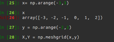
    shift_x, shift_y = xp.meshgrid(shift_x, shift_y)   #shift_x = [[0，16，32，..],[0，16，32，..],[0，16，32，..]...],shift_x = [[0，0，0，..],[16，16，16，..],[32，32，32，..]...],就是形成了一个纵横向偏移量的矩阵，也就是特征图的每一点都能够通过这个矩阵找到映射在原图中的具体位置！
#产生的大X 以x的行为行，以y的元素个数为列构成矩阵，同样的产生的Y以y的行作为列，以x的元素个数作为列数产生矩阵
    shift = xp.stack((shift_y.ravel(), shift_x.ravel(),
                      shift_y.ravel(), shift_x.ravel()), axis=1)  #经过刚才的变化，其实大X,Y的元素个数已经相同，看矩阵的结构也能看出，矩阵大小是相同的，X.ravel()之后变成一行，此时shift_x,shift_y的元素个数是相同的，都等于特征图的长宽的乘积(像素点个数)，不同的是此时的shift_x里面装得是横向看的x的一行一行的偏移坐标，而此时的y里面装得是对应的纵向的偏移坐标！下图显示xp.meshgrid（），shift_y.ravel()操作示例
    A = anchor_base.shape[0] #A=9
    K = shift.shape[0] #读取特征图中元素的总个数
    anchor = anchor_base.reshape((1, A, 4)) + \
             shift.reshape((1, K, 4)).transpose((1, 0, 2))    #用基础的9个anchor的坐标分别和偏移量相加，最后得出了所有的anchor的坐标，四列可以堪称是左上角的坐标和右下角的坐标加偏移量的同步执行，飞速的从上往下捋一遍，所有的anchor就都出来了！一共K个特征点，每一个有A(9)个基本的anchor，所以最后reshape((K*A),4)的形式，也就得到了最后的所有的anchor左下角和右上角坐标.          
    anchor = anchor.reshape((K * A, 4)).astype(np.float32)
    return anchor

下面是shift_x, shift_y = xp.meshgrid(shift_x, shift_y)函数操作示意图


shift = xp.stack((shift_y.ravel(), shift_x.ravel(),shift_y.ravel(), shift_x.ravel()), axis=1)主要是产生偏移坐标对，一个朝x方向，一个朝y方向偏移。给’‘特征图’'上每个点对应都画与anchor_base一样的框，得到每个框的左上角和右下角坐标。

还有一个问题就是为什么要将特征图对应回原图的大小呢？因为你要框住的待检测目标是在原图，而你选取anchor是在特征图上，pooling之后特征之间的相对位置不变，但是尺寸缩小为原来的1/16,也就是说，一个点对应于原图的16个点的信息，原图和特征图对应的感受野是不一样的，而你的anchor目的是为了框原图的目标的，如果不remap回原图的话，你一个base_size的anchor基本就框住了特征图的大部分的信息，这样的目标检测没有任何意义的，论文作者之所以采用这种网络结构其中一个目的也是为了让特征图和原图的对应关系明确，方便remap回原图从而选取anchor，产生proposal!

接下来再看的是model/creator_tool.py文件
这个脚本实现了三个Creator函数，分别是：ProposalCreator、AnchorTargetCreator、ProposalTargetCreator
前两个都在RPN网络里实现，第三个在RoIHead网络里实现。

AnchorTargetCreator：
目的：利用每张图中bbox的真实标签来为所有任务分配ground truth！

输入：最初生成的20000个anchor坐标、此一张图中所有的bbox的真实坐标

输出：size为（20000，1）的正负label（其中只有128个为1，128个为0，其余都为-1）、 size为（20000，4）的回归目标（所有anchor的坐标都有）

前面讲到每张图进来都会生成约20000个anchor，前面已经分析了这20000个anchor的生成过程。那问题来了，我们在RPN网络里要做三个操作：分类、回归、提供rois 。分类和回归的ground truth 怎么获取？如何给20000个anchor在分类时赋予正负标签gt_rpn_label？如何给回归操作赋予回归目标gt_rpn_loc？？？ 这就是此creator的目的，利用每张图bbox的真实标签来为所有任务分配ground truth！

注意虽然是给所有20000个anchor赋予了ground truth，但是我们只从中任挑128个正类和128个负类共256个样本来训练。不利用所有样本训练的原因是显然图中负类远多于正类样本数目。同样回归也只挑256个anchor来完成。

此函数首先将一张图中所有20000个anchor中所有完整包含在图像中的anchor筛选出来，假如挑出15000个anchor，要记录下来这部分的索引。

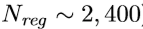
然后利用函数bbox_iou计算15000个anchor与真实bbox的IOU。然后利用函数_create_label根据行列索引分别求出每个anchor与哪个bbox的iou最大，以及最大值，然后返回最大iou的索引argmax_ious(即每个anchor与真实bbox最大iou的索引)与label（label中背景为-1，负样本为0， 正样本为1）。注意虽然是要挑选256个，但是这里返回的label仍然是全部，只不过label里面有128为0，128个为1，其余都为-1而已。然后函数bbox2loc利用返回的索引argmax_ious来计算出回归的目标参数组loc。然后根据之前记录的索引，将15000个再映射回20000长度的label（其余的label一律置为-1）和loc（其余的loc一律置为（0，0，0，0））。有了RPN网络两个11卷积输出的类别label和位置参数loc的预测值，AnchorTargetCreator又为其对应生成了真实值ground truth。那么AnchorTargetCreator的损失函数rpn_loss就很了然了：

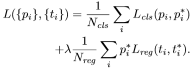
cls代表二分类，reg代表回归。为什么我们挑出来256个label还要映射回20000呢？就是因为这里网络的预测结果（11卷积）就是20000个，而我们将要忽略的label都设为了-1，这就允许我们得以筛选，而loc也是一样的道理。所以损失函数里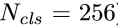

#下面是ProposalCreator的代码： 这部分的操作不需要进行反向传播，因此可以利用numpy/tensor实现
class ProposalCreator: #对于每张图片，利用它的feature map，计算（H/16）x(W/16)x9(大概20000)个anchor属于前景的概率，然后从中选取概率较大的12000张，利用位置回归参数，修正这12000个anchor的位置， 利用非极大值抑制，选出2000个ROIS以及对应的位置参数。
    def __call__(self, loc, score,anchor, img_size, scale=1.):  #这里的loc和score是经过region_proposal_network中经过1x1卷积分类和回归得到的
        if self.parent_model.training:  
        n_pre_nms = self.n_train_pre_nms #12000
            n_post_nms = self.n_train_post_nms #经过NMS后有2000个
        else:
            n_pre_nms = self.n_test_pre_nms #6000
            n_post_nms = self.n_test_post_nms #经过NMS后有300个
        roi = loc2bbox(anchor, loc) #将bbox转换为近似groudtruth的anchor(即rois)
        roi[:, slice(0, 4, 2)] = np.clip( roi[:, slice(0, 4, 2)], 0, img_size[0]) #裁剪将rois的ymin,ymax限定在[0,H]
        roi[:, slice(1, 4, 2)] = np.clip(roi[:, slice(1, 4, 2)], 0, img_size[1]) #裁剪将rois的xmin,xmax限定在[0,W]

        min_size = self.min_size * scale   #16
        hs = roi[:, 2] - roi[:, 0] #rois的宽
        ws = roi[:, 3] - roi[:, 1] #rois的长
        keep = np.where((hs >= min_size) & (ws >= min_size))[0] #确保rois的长宽大于最小阈值
        roi = roi[keep, :]
        score = score[keep] #对剩下的ROIs进行打分（根据region_proposal_network中rois的预测前景概率）
        
        order = score.ravel().argsort()[::-1]  #将score拉伸并逆序（从高到低）排序
        if n_pre_nms > 0:
            order = order[:n_pre_nms] #train时从20000中取前12000个rois，test取前6000个
        roi = roi[order, :]

        keep = non_maximum_suppression(
            cp.ascontiguousarray(cp.asarray(roi)),
            thresh=self.nms_thresh)  #（具体需要看NMS的原理以及输入参数的作用）调用非极大值抑制函数，将重复的抑制掉，就可以将筛选后ROIS进行返回。经过NMS处理后Train数据集得到2000个框，Test数据集得到300个框
        if n_post_nms > 0:
            keep = keep[:n_post_nms]
        roi = roi[keep]
        return roi 取出最终的2000或300个rois

#下面是AnchorTargetCreator（）代码，作用是生成训练要用的anchor(与对应框iou值最大或者最小的各128个框的坐标和256个label（0或者1）)
class AnchorTargetCreator(object): #利用每张图中bbox的真实标签来为所有任务分配ground truth！
#为Faster-RCNN专有的RPN网络提供自我训练的样本，RPN网络正是利用AnchorTargetCreator产生的样本作为数据进行网络的训练和学习的，这样产生的预测anchor的类别和位置才更加精确，anchor变成真正的ROIS需要进行位置修正，而AnchorTargetCreator产生的带标签的样本就是给RPN网络进行训练学习用哒
    def __call__(self, bbox, anchor, img_size): #anchor:(S,4),S为anchor数
        img_H, img_W = img_size
        n_anchor = len(anchor)  #一般对应20000个左右anchor
        inside_index = _get_inside_index(anchor, img_H, img_W) #将那些超出图片范围的anchor全部去掉,只保留位于图片内部的序号
        anchor = anchor[inside_index] #保留位于图片内部的anchor
        argmax_ious, label = self._create_label( inside_index, anchor, bbox)  #筛选出符合条件的正例128个负例128并给它们附上相应的label
        loc = bbox2loc(anchor, bbox[argmax_ious])  #计算每一个anchor与对应bbox求得iou最大的bbox计算偏移量（注意这里是位于图片内部的每一个）
        label = _unmap(label, n_anchor, inside_index, fill=-1)  #将位于图片内部的框的label对应到所有生成的20000个框中（label原本为所有在图片中的框的）
        loc = _unmap(loc, n_anchor, inside_index, fill=0) #将回归的框对应到所有生成的20000个框中（label原本为所有在图片中的框的）
        return loc, label
        
#下面为调用的_creat_label（） 函数
     def _create_label(self, inside_index, anchor, bbox):
        label = np.empty((len(inside_index),), dtype=np.int32)           #inside_index为所有在图片范围内的anchor序号
        label.fill(-1)   #全部填充-1
        argmax_ious, max_ious, gt_argmax_ious = self._calc_ious(anchor, bbox, inside_index)调用_calc_ious（）函数得到每个anchor与哪个bbox的iou最大以及这个iou值、每个bbox与哪个anchor的iou最大(需要体会从行和列取最大值的区别)
        label[max_ious < self.neg_iou_thresh] = 0 #把每个anchor与对应的框求得的iou值与负样本阈值比较，若小于负样本阈值，则label设为0，pos_iou_thresh=0.7, neg_iou_thresh=0.3
        label[gt_argmax_ious] = 1   #把与每个bbox求得iou值最大的anchor的label设为1
        label[max_ious >= self.pos_iou_thresh] = 1  ##把每个anchor与对应的框求得的iou值与正样本阈值比较，若大于正样本阈值，则label设为1
        n_pos = int(self.pos_ratio * self.n_sample) #按照比例计算出正样本数量，pos_ratio=0.5，n_sample=256
        pos_index = np.where(label == 1)[0]  #得到所有正样本的索引
        if len(pos_index) > n_pos:         #如果选取出来的正样本数多于预设定的正样本数，则随机抛弃，将那些抛弃的样本的label设为-1
            disable_index = np.random.choice(
                pos_index, size=(len(pos_index) - n_pos), replace=False)
            label[disable_index] = -1
        n_neg = self.n_sample - np.sum(label == 1) #设定的负样本的数量
        neg_index = np.where(label == 0)[0]  #负样本的索引
        if len(neg_index) > n_neg:
            disable_index = np.random.choice(
                neg_index, size=(len(neg_index) - n_neg), replace=False)  #随机选择不要的负样本，个数为len(neg_index)-neg_index，label值设为-1
            label[disable_index] = -1 
        return argmax_ious, label

#下面为调用的_calc_ious（）函数        
    def _calc_ious(self, anchor, bbox, inside_index):
        ious = bbox_iou(anchor, bbox)    #调用bbox_iou函数计算anchor与bbox的IOU， ious：（N,K），N为anchor中第N个，K为bbox中第K个，N大概有15000个
        argmax_ious = ious.argmax(axis=1)   #1代表行，0代表列
        max_ious = ious[np.arange(len(inside_index)), argmax_ious] #求出每个anchor与哪个bbox的iou最大，以及最大值，max_ious:[1,N]
        gt_argmax_ious = ious.argmax(axis=0)
        gt_max_ious = ious[gt_argmax_ious, np.arange(ious.shape[1])] #求出每个bbox与哪个anchor的iou最大，以及最大值,gt_max_ious:[1,K]
        gt_argmax_ious = np.where(ious == gt_max_ious)[0]   #然后返回最大iou的索引（每个bbox与哪个anchor的iou最大),有K个

下面是ProposalTargetCreator的代码：
目的：为2000个rois赋予ground truth！（严格讲挑出128个赋予ground truth！）

输入：2000个rois、一个batch（一张图）中所有的bbox ground truth（R，4）、对应bbox所包含的label（R，1）（VOC2007来说20类0-19）

输出：128个sample roi（128，4）、128个gt_roi_loc（128，4）、128个gt_roi_label（128，1）

ProposalCreator 输出的2000个roi作为ProposalTargetCreator的输入，同时输入的还有一张图上的所有bbox、label的ground trurh。如果此输入图像里有5个object，那么就有5个bbox和5个label。那么这时的三个输入可能是：下面我们将使用此例R=5来分析：

这三个分别为 5x4 bbox的ground truth , 5x1 label , 2000x4个roi

#下面是ProposalTargetCreator代码：ProposalCreator产生2000个ROIS，但是这些ROIS并不都用于训练，经过本ProposalTargetCreator的筛选产生128个用于自身的训练
class ProposalTargetCreator(object):  #为2000个rois赋予ground truth！（严格讲挑出128个赋予ground truth！）
#输入：2000个rois、一个batch（一张图）中所有的bbox ground truth（R，4）、对应bbox所包含的label（R，1）（VOC2007来说20类0-19）
#输出：128个sample roi（128，4）、128个gt_roi_loc（128，4）、128个gt_roi_label（128，1）
    def __call__(self, roi, bbox, label, loc_normalize_mean=(0., 0., 0., 0.), loc_normalize_std=(0.1, 0.1, 0.2, 0.2)):  #因为这些数据是要放入到整个大网络里进行训练的，比如说位置数据，所以要对其位置坐标进行数据增强处理(归一化处理)
        n_bbox, _ = bbox.shape
        roi = np.concatenate((roi, bbox), axis=0) #首先将2000个roi和m个bbox给concatenate了一下成为新的roi（2000+m，4）。
        pos_roi_per_image = np.round(self.n_sample * self.pos_ratio)  #n_sample = 128,pos_ratio=0.5，round 对传入的数据进行四舍五入
        iou = bbox_iou(roi, bbox) #计算每一个roi与每一个bbox的iou
        gt_assignment = iou.argmax(axis=1) #按行找到最大值，返回最大值对应的序号以及其真正的IOU。返回的是每个roi与**哪个**bbox的最大，以及最大的iou值
        max_iou = iou.max(axis=1) #每个roi与对应bbox最大的iou
        gt_roi_label = label[gt_assignment] + 1 #从1开始的类别序号，给每个类得到真正的label(将0-19变为1-20)
        pos_index = np.where(max_iou >= self.pos_iou_thresh)[0]  #同样的根据iou的最大值将正负样本找出来，pos_iou_thresh=0.5
        pos_roi_per_this_image = int(min(pos_roi_per_image, pos_index.size))   #需要保留的roi个数（满足大于pos_iou_thresh条件的roi与64之间较小的一个）
        if pos_index.size > 0:
            pos_index = np.random.choice(
                pos_index, size=pos_roi_per_this_image, replace=False)  #找出的样本数目过多就随机丢掉一些

        neg_index = np.where((max_iou < self.neg_iou_thresh_hi) &
                             (max_iou >= self.neg_iou_thresh_lo))[0]  #neg_iou_thresh_hi=0.5，neg_iou_thresh_lo=0.0
        neg_roi_per_this_image = self.n_sample - pos_roi_per_this_image # #需要保留的roi个数（满足大于0小于neg_iou_thresh_hi条件的roi与64之间较小的一个）
        neg_roi_per_this_image = int(min(neg_roi_per_this_image,
                                         neg_index.size))
        if neg_index.size > 0:
            neg_index = np.random.choice(
                neg_index, size=neg_roi_per_this_image, replace=False)  #找出的样本数目过多就随机丢掉一些

        keep_index = np.append(pos_index, neg_index)
        gt_roi_label = gt_roi_label[keep_index]
        gt_roi_label[pos_roi_per_this_image:] = 0  # 负样本label 设为0
        sample_roi = roi[keep_index]
#那么此时输出的128*4的sample_roi就可以去扔到 RoIHead网络里去进行分类与回归了。同样， RoIHead网络利用这sample_roi+featue为输入，输出是分类（21类）和回归（进一步微调bbox）的预测值，那么分类回归的groud truth就是ProposalTargetCreator输出的gt_roi_label和gt_roi_loc。
        gt_roi_loc = bbox2loc(sample_roi, bbox[gt_assignment[keep_index]]) #求这128个样本的groundtruth
        gt_roi_loc = ((gt_roi_loc - np.array(loc_normalize_mean, np.float32)
                       ) / np.array(loc_normalize_std, np.float32))  #ProposalTargetCreator首次用到了真实的21个类的label,且该类最后对loc进行了归一化处理，所以预测时要进行均值方差处理
        return sample_roi, gt_roi_loc, gt_roi_label