


不想干正事练习点别的。

来自kaggle项目:
Visualizing Pokémon Stats with Seaborn
EDA-Pokemon
目录
Part1: 探索性数据分析:
1)特征分析.
2)发现特征间的关系和趋势
Part2: 特征工程和数据清洗:
1)移除多余的特征
2)数据类型的转换
Part3: 预测模型
1)基本算法
2)交叉验证
3)集成算法
4)重要特征抽取
Part1: 探索性数据分析:
导入库
import pandas as pd
import seaborn as sns
import matplotlib.pyplot as plt
输入数据
data = pd.read_csv("C:\\Users\\Nihil\\Documents\\pythonlearn\\data\\kaggle\\Pokemon.csv")
我从kaggle直接下载的数据有乱码,解决方法:
把文件另存为编码utf-8即可。
pd.set_option('display.max_columns', 1000)
pd.set_option('display.width', 1000)
pd.set_option('display.max_colwidth', 1000)
print(data.head())

数据包括了:
小精灵的名字,
类型,
不同的属性值,
还有一个Total变量。
- 每个数据的含义
#ID:每个宠物小精灵的ID
名称:每个口袋妖怪的名字
属性1:每个口袋妖怪都有一个属性,这决定了他们的克制与被克制关系
属性2:还有一些口袋妖怪是双重属性的
总计:所有的统计数据的总和,某种程度上决定了精灵的强弱
HP:生命值,在被击倒之前宠物小精灵可以承受多少的伤害
攻击:物理攻击的基础数值(例如Scratch,Punch)
防御:抵抗物理攻击的基础数值
SP攻击:特殊攻击,特殊攻击的基础数值(例如火焰爆炸,泡沫射线)
SP Def:抵抗特殊攻击的基础数值
速度:决定宠物小精灵的进攻顺序
世代: 该精灵在第几世代中出现
神兽: 该精灵是否为神兽(Label)
变量相关性——采用jointplot
参考:Seaborn分布数据可视化
作用: seaborn会直接给出变量的皮尔逊相关系数和P值
基于HP和Attack
sns.jointplot(x='HP',y='Attack',data=data)
plt.show()
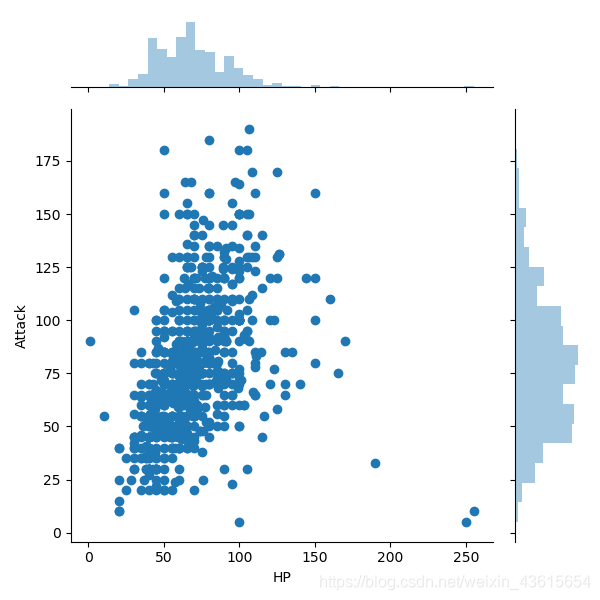
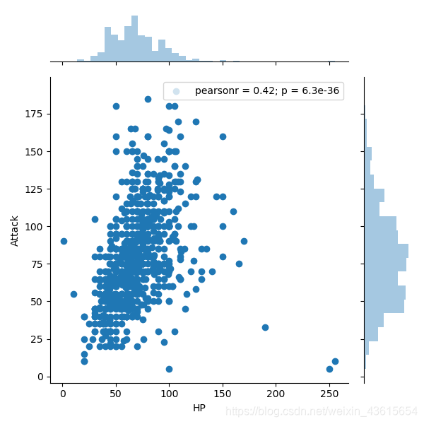
发现没显示皮尔逊相关系数和P值,所以修改了一下代码
#增加
import scipy.stats as stats
from warnings import filterwarnings
filterwarnings('ignore')

sns.jointplot(x='HP',y='Attack',data=data).annotate(stats.pearsonr)
plt.show()
理解:如何通俗易懂地理解皮尔逊相关系数?
统计学三大相关系数之皮尔森(pearson)相关系数
读懂Pearson相关分析结果
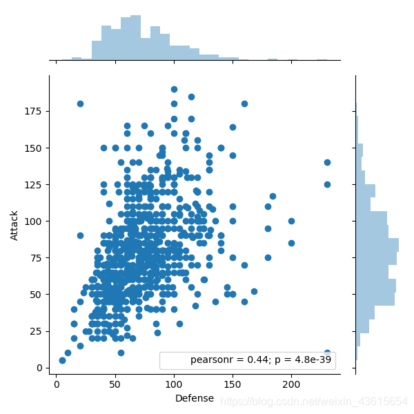
换成攻击和防御试试
sns.jointplot(x='Defense',y='Attack',data=data).annotate(stats.pearsonr)
plt.show()
结果:
识别异常值——采用Boxplot
采用Boxplot看六种属性的分布。
- Boxplot的资料
eaborn学习笔记1——箱形图Boxplot
Boxplot的含义
优点:箱型图选取异常值比较客观,在识别异常值方面有一定的优越性。
数据预处理之异常值处理
sns.boxplot(data=data)
plt.show()
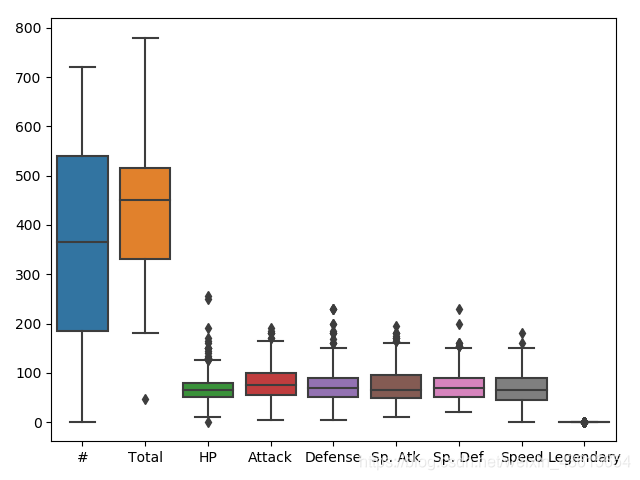
从图中可看出,我们可以去掉ID和所有的统计数据的总和。
data = data.drop(['Total','#'],axis=1)
print(data.head(5))

#运行结果
                    Name Type 1  Type 2  HP  Attack  Defense  Sp. Atk  Sp. Def  Speed Generation Legendary
0              Bulbasaur  Grass  Poison  45      49       49       65       65     45          1     False
1                Ivysaur  Grass  Poison  60      62       63       80       80     60          1     False
2               Venusaur  Grass  Poison  80      82       83      100      100     80          1     False
3  VenusaurMega Venusaur  Grass  Poison  80     100      123      122      120     80          1     False
4             Charmander   Fire     NaN  39      52       43       60       50     65          1     False
把#留下当索引,并去掉其名称。
data = data.set_index('#')
print(data.head(5))

#results
                    Name Type 1  Type 2  HP  Attack  Defense  Sp. Atk  Sp. Def  Speed Generation Legendary
#
1              Bulbasaur  Grass  Poison  45      49       49       65       65     45          1     False
2                Ivysaur  Grass  Poison  60      62       63       80       80     60          1     False
3               Venusaur  Grass  Poison  80      82       83      100      100     80          1     False
3  VenusaurMega Venusaur  Grass  Poison  80     100      123      122      120     80          1     False
4             Charmander   Fire     NaN  39      52       43       60       50     65          1     False
pandas中关于set_index和reset_index的用法
data.index.name = ''

#Results
                   Name Type 1  Type 2  HP  Attack  Defense  Sp. Atk  Sp. Def  Speed Generation Legendary

1              Bulbasaur  Grass  Poison  45      49       49       65       65     45          1     False
2                Ivysaur  Grass  Poison  60      62       63       80       80     60          1     False
3               Venusaur  Grass  Poison  80      82       83      100      100     80          1     False
3  VenusaurMega Venusaur  Grass  Poison  80     100      123      122      120     80          1     False
4             Charmander   Fire     NaN  39      52       43       60       50     65          1     False
检查缺失值
print(data.isnull().sum())

#Results
Name            0
Type 1          1
Type 2        385
HP              0
Attack          0
Defense         0
Sp. Atk         0
Sp. Def         0
Speed           0
Generation      0
Legendary       1
dtype: int64
Tpye2有386个缺失值。
不知道为啥我下载的数据集少了一个,算了缺一个也无视了。下次再看看缺失值处理方面的。
查看Legendary占比(label)
f,ax = plt.subplots(1,2,figsize=(15,8))

data['Legendary'].value_counts().plot.pie(ax=ax[0],shadow=True,explode=[0,0.1],autopct='%1.1f%%')
ax[0].set_ylabel('')
ax[0].set_xlabel('Legendary')
sns.countplot('Legendary',data=data,ax=ax[1])
ax[1].set_ylabel('')
ax[1].set_xlabel('Legendary')
plt.show()
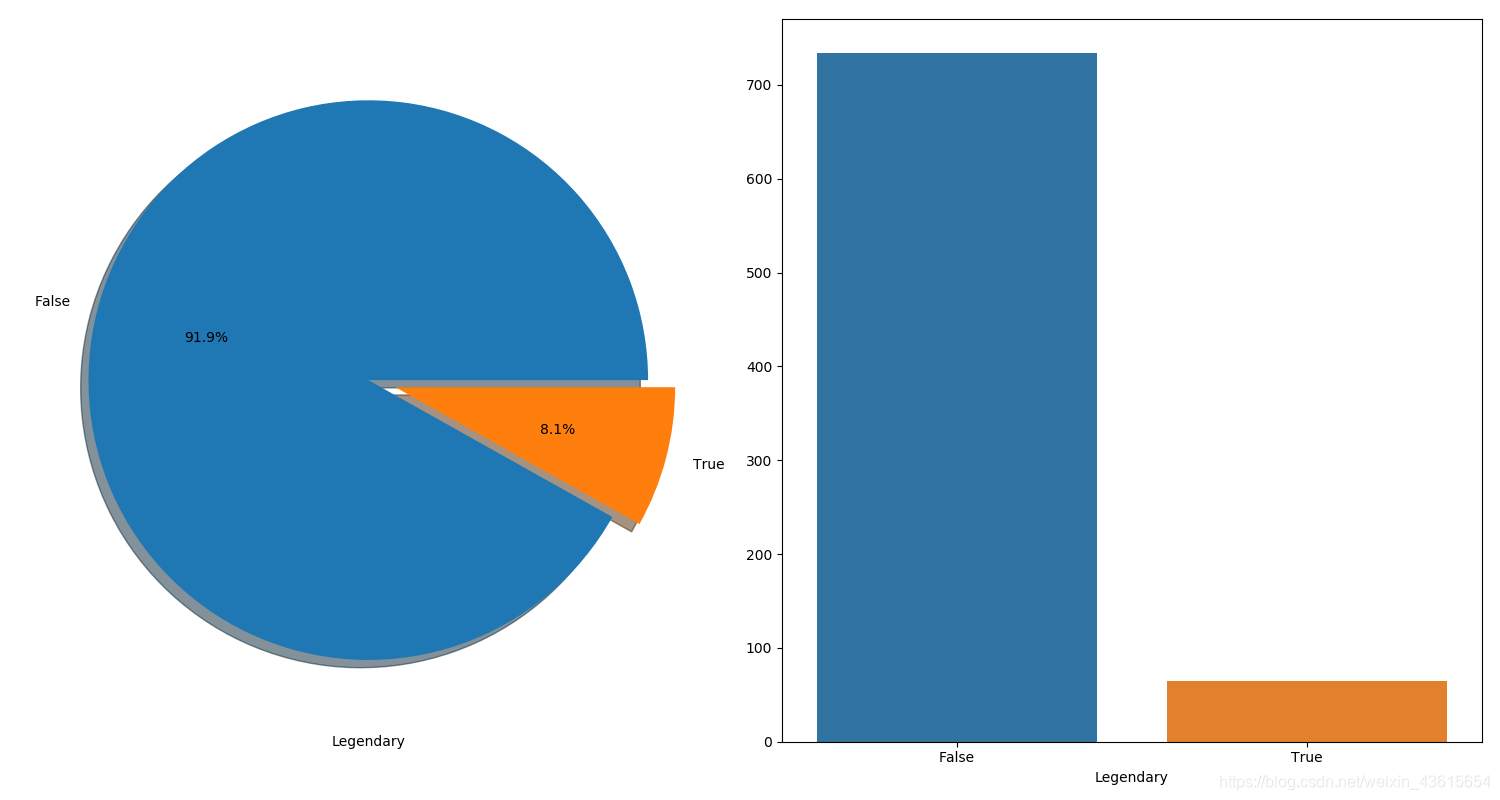
数据极不平衡,True远远小于False。
了解数据类型
print(data.info())
print(data.isnull().sum())

Data columns (total 11 columns):
Name          800 non-null object
Type 1        799 non-null object
Type 2        415 non-null object
HP            800 non-null int64
Attack        800 non-null int64
Defense       800 non-null int64
Sp. Atk       800 non-null int64
Sp. Def       800 non-null int64
Speed         800 non-null int64
Generation    800 non-null object
Legendary     799 non-null object
dtypes: int64(6), object(5)
memory usage: 75.0+ KB
print(data.describe())

#results
               HP      Attack     Defense     Sp. Atk     Sp. Def       Speed
count  800.000000  800.000000  800.000000  800.000000  800.000000  800.000000
mean    69.272500   78.980000   73.842500   72.820000   71.915000   68.216250
std     25.525089   32.477347   31.183501   32.722294   27.816811   29.150543
min      1.000000    5.000000    5.000000   10.000000   20.000000    1.000000
25%     50.000000   55.000000   50.000000   49.750000   50.000000   45.000000
50%     65.000000   75.000000   70.000000   65.000000   70.000000   65.000000
75%     80.000000  100.000000   90.000000   95.000000   90.000000   90.000000
max    255.000000  190.000000  230.000000  194.000000  230.000000  180.000000
输出分类特征(Categorical Features):Name,Type 1,Type 2
print(data.describe(include=['O']))
Python pandas.DataFrame.describe函数方法的使用
pandas 的describe函数的参数详解
输出结果:
                       Name Type 1  Type 2 Generation Legendary
count                   800    799     415        800       799
unique                  800     18      19          7         2
top     PumpkabooSuper Size  Water  Flying          1     False
freq                      1    112      97        165       734

可以看出describe(include=['O']的作用是输出字符串类型的结果
发现Generation,Legendary也算成了object,整了一晚上转换数据类型也是失败。当然可以参照一些:
pandas 数据类型转换
Pandas数据类型转换的几个小技巧
真实错误的原因:
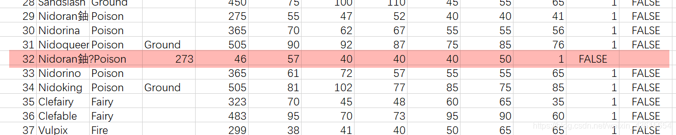
行吧直接删掉这行。
所以一定要好好大致检查一下数据。
data['Generation'] = pd.to_numeric(data['Generation'],errors="ignore")
print(data['Generation'].dtypes)

#Results
int64

print(data.describe(include=['O']))
                         Name Type 1  Type 2
count                     798    798     414
unique                    798     18      18
top     CameruptMega Camerupt  Water  Flying
freq                        1    112      97
OK.
序数特征(Ordinal Features):Generation
print(data.Generation.value_counts())

#Results
5    165
1    164
3    160
4    121
2    106
6     82
Name: Generation, dtype: int64
连续性特征(Continous Feature)
- HP
- Attack
- Defense
- Sp. Atk
- Sp. Def
- Speed
- 特征分析
分类特征分析
- Type 1–> 分类特征
out = data[['Type 1','Legendary']].groupby('Type 1').count()
print(out)

#Result
         Legendary
Type 1
Bug              69
Dark             31
Dragon           32
Electric         44
Fairy            17
Fighting         27
Fire             52
Flying            4
Ghost            32
Grass            70
Ground           32
Ice              24
Normal           98
Poison           26
Psychic          57
Rock             44
Steel            27
Water           112
属性1:每个口袋妖怪都有一个属性,这决定了他们的克制与被克制关系,因此绘制一个统计图(哪种属性会导致某种标签结果)
f,ax = plt.subplots(1,2,figsize=(18,8))
data[['Type 1','Legendary']].groupby('Type 1').mean().plot.bar(ax=ax[0])
ax[0].set_title('type1 vs Legendary')
sns.countplot('Type 1',hue='Legendary',data=data,ax=ax[1])
plt.show()
- 我总是犯的错: 多图subplots记得加s
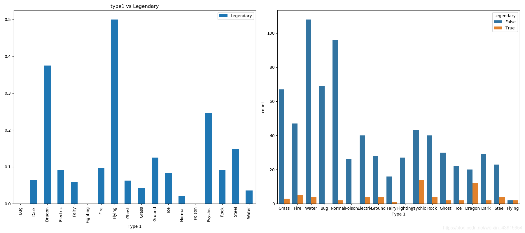
可以粗略看出Dragon,flying和psychic称为神兽的可能性较高,尤其会飞
分类型特征分析(Type2)
out = data[['Type 2']].describe()
print(out)
#Results
        Type 2
count      414
unique      18
top     Flying
freq        97
Type2的缺失值过多,移除
——写了一下午的东西没了无语,我讨厌Chrome——

回一下血,今天继续重新肝。
序列特征分析
- 用crosstab检验
交叉表是用于统计分组频率的特殊透视表
关于crosstab的使用Pandas:透视表(pivotTab)和交叉表(crossTab)
out = pd.crosstab(data.Generation,data.Legendary,margins=True)
print(out)

#Results
Legendary   False  True  All
Generation
1             158     6  164
2             101     5  106
3             142    18  160
4             108    13  121
5             150    15  165
6              74     8   82
All           733    65  798
查看比例:
plt.rcParams['font.sans-serif']=['SimHei']
f,ax=plt.subplots(1,2,figsize=(18,8))
data['Generation'].value_counts().plot.bar(ax=ax[0])
ax[0].set_ylabel('countS')
ax[0].set_title('Generation')
sns.countplot('Generation',hue='Legendary',data=data,ax=ax[1])
ax[1].set_title('Legendary VS Generation')
print("第三代神兽比例: ", round(18/160,2))
print("第四代神兽比例: ", round(13/121,2))
print("第五代神兽比例: ", round(15/165,2))
print("第六代神兽比例: ", round(8/82,2))
plt.show()

#Results
第三代神兽比例:  0.11
第四代神兽比例:  0.11
第五代神兽比例:  0.09
第六代神兽比例:  0.1
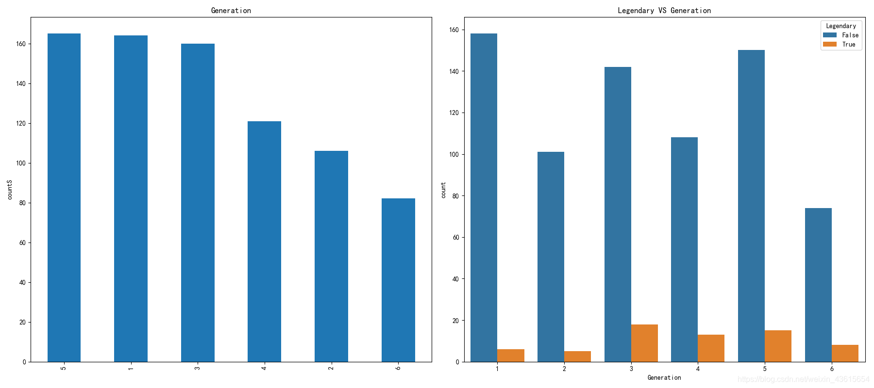
可以看出,3代和4代更容易出神兽。
连续性特征
对于连续值,主要看其分布。
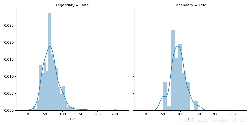
HP
属性含义: 生命值,被击倒之前宠物小精灵可以承受多少的伤害
g = sns.FacetGrid(data, col='Legendary',size=5)
g = g.map(sns.distplot, "HP")
plt.show()
plt.figure(figsize=(15,8))
g = sns.kdeplot(data["HP"][data["Legendary"] == False], color="Red", shade = True)
g = sns.kdeplot(data["HP"][data["Legendary"] == True], ax =g, color="Blue", shade= True)
g.set_xlabel("HP")
g.set_ylabel("Frequency")
g = g.legend(["not Legendary","Legendary"])
print('not Legendary HP:',data["HP"][data["Legendary"] == 0].value_counts().index[0])
print('Legendary HP:',data["HP"][data["Legendary"] == 1].value_counts().index[0])
plt.show()
Note:
1.这里[data[“Legendary”] == False]与data[“HP”][data[“Legendary”] == 0一样,反正我都用了没什么差别。
2.ax =g用和不用效果一样。
3.index[0]显示频次最高的
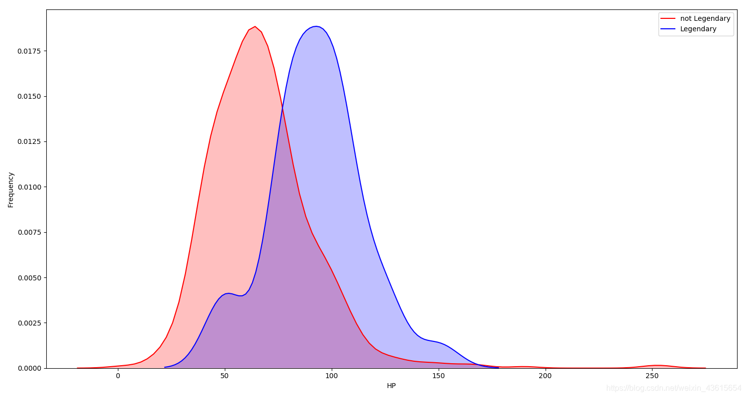
运行结果:
not Legendary HP: 60
Legendary HP: 100
之后几个连续特征按照这个思路就行。昨天写得都崩了。就不再全部弄一遍了。结果为:
not Legendary Attack: 65
Legendary Attack: 100
not Legendary Defense: 70
Legendary Defense在: 90
not Legendary Sp. Atk: 60
Legendary Sp. Atk: 150
not Legendary Sp. Def: 50
Legendary Sp. Def: 90
not Legendary Speed: 50
Legendary Speed: 90
显然,神兽各属性值都算比较高的(要不怎么是神兽?

接下来是分析序列特征里连续特征的分布(拗口
sns.factorplot('Generation','Sp. Atk',hue='Legendary',data=data,size=8)
plt.show()
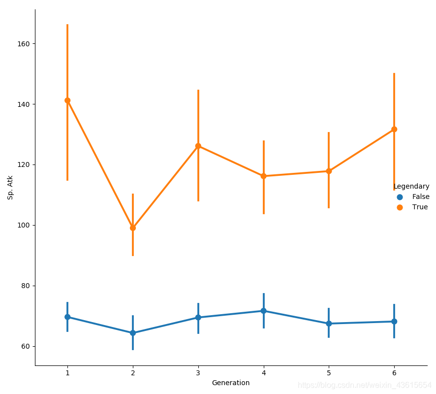
从图上基本可以清晰的获取以下信息:
2代的攻击最低。
1代攻击最高并且浮动较大。
更显然的看到神兽的属性值很高。
继续深入以下,关于factorplot,参考了使用 seaborn 的 FacetGrid 绘图的方法
代码:
grid = sns.FacetGrid(data, col='Generation', hue='Legendary', palette='seismic', size=4)
grid.map(sns.countplot, 'Sp. Atk', alpha=.8)
grid.add_legend()
plt.show()
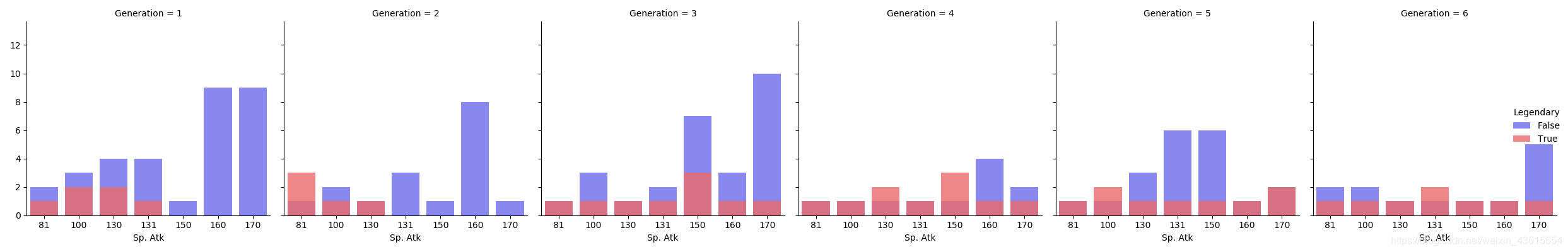
从这张图可以知道:一代里特殊攻击高的最多。而且都是非神兽。但特殊攻击最高的还是第三代。一代神兽特殊攻击分布比较散。
其余几个连续值继续照着这个思路分析一遍。
特征的相关性
思路:获取数据后,需要求特征的相关系数。可以用padas直接求出来相关系数,放到heatmap,可以很清楚的看到两个特征的相关程度。
用途:比如拿到一批离散数据,想看一下在哪个点值比较大,在哪个点值比较低,你想把这样一个值的变化,用颜色来区分出来,这是我们要做的一个变化
plt.figure(figsize=(10,10))
sns.heatmap(data.drop(['Name','Legendary'],axis=1).corr(),annot=True)
plt.show()
资料囤积:
seaborn.heatmap参数介绍
相关系数矩阵与热力图heatmap(Python高级可视化库seaborn)
调色
外:
Seaborn Heatmap Tutorial (Python Data Visualization)
Day (4) — Data Visualization — How to use Seaborn for Heatmaps
运行结果:
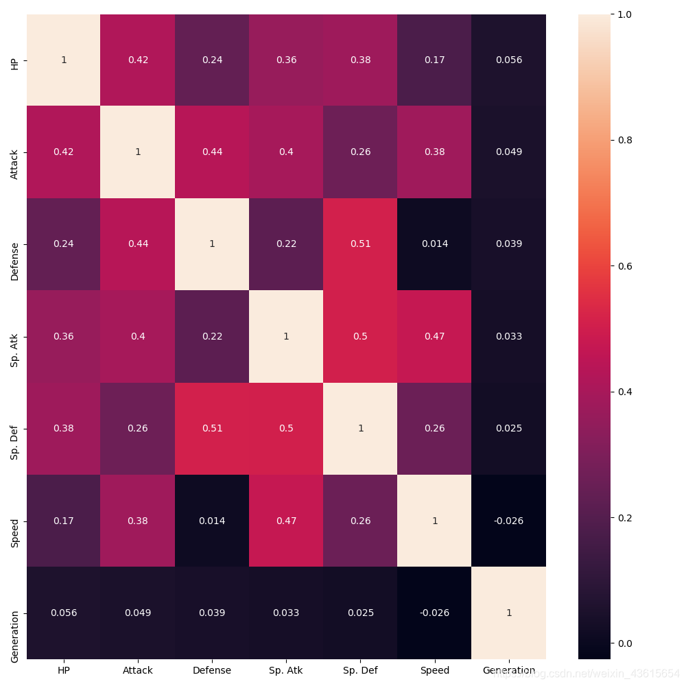
可以看出基本都没啥关系。
Part2: 特征工程和清洗数据
去掉多余特征
- 'Name’是小精灵的名字
- 'Type 2’缺失数据太多
data.drop(['Name','Type 2'],axis=1,inplace=True)
转换数据类型
Type 1
看看类型1有哪些类型
out = data['Type 1'].value_counts().index
print(out)

#Results
Index(['Water', 'Normal', 'Grass', 'Bug', 'Psychic', 'Fire', 'Electric', 'Rock', 'Ground', 'Ghost', 'Dragon', 'Dark', 'Fighting', 'Steel', 'Poison', 'Ice', 'Fairy', 'Flying'], dtype='object')
把文字标签换成数字标签。
Replace:
pandas的替换和部分替换(replace)
data['Type 1'].replace(['Water', 'Normal', 'Grass', 'Bug', 'Psychic', 'Fire',
                        'Rock','Electric', 'Ground', 'Dragon', 'Ghost', 'Dark',
                        'Poison', 'Steel','Fighting', 'Ice', 'Fairy', 'Flying'],list(range(1,19)),inplace=True)
print(data['Type 1'].value_counts().index)

#Results
Int64Index([1, 2, 3, 4, 5, 6, 8, 7, 9, 10, 11, 12, 14, 15, 13, 16, 17, 18], dtype='int64')
同样的,把Legendary也换成数字。
查看:
out = data['Legendary'].value_counts().index
print(out)

#Result:
Index([False, True], dtype='object')
由于Legendary的取值较少(1,0),直接采用map函数就行。
out = data['Legendary']=data['Legendary'].map({False:0,True:1})
print(out)
map函数的一些用法
python 中map()函数的使用方法
Python map() function
现在可以再检查一遍相关性了
plt.figure(figsize=(10,10))
sns.heatmap(data.corr(),annot=True,cmap='Greens')
plt.show()
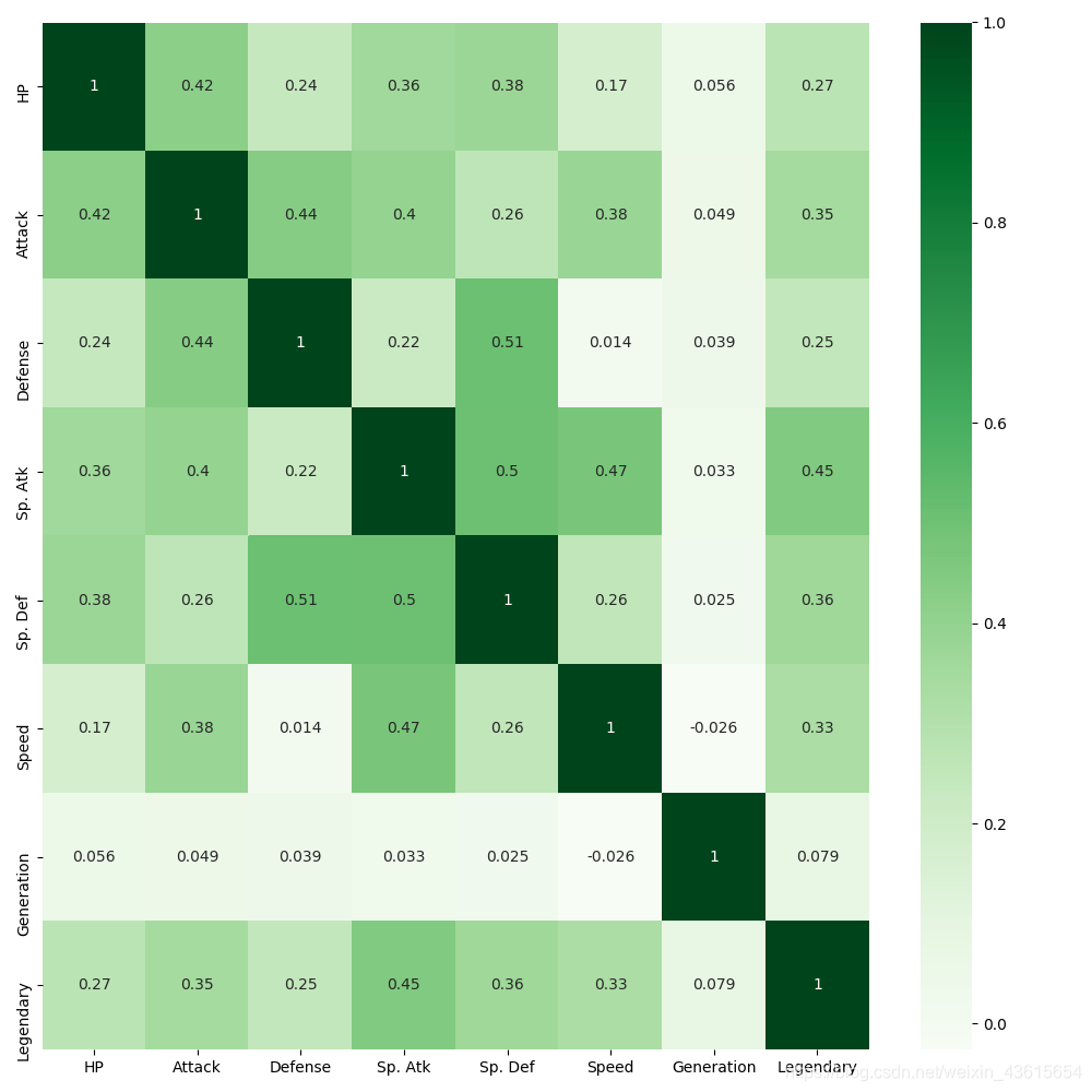
这图说明了:能成为神兽最大关系都在于特殊攻击。

最后检查一下数据
print(data.head(5))

#Results
  Type 1  HP  Attack  Defense  Sp. Atk  Sp. Def  Speed  Generation  Legendary

1  Grass  45      49       49       65       65     45           1          0
2  Grass  60      62       63       80       80     60           1          0
3  Grass  80      82       83      100      100     80           1          0
3  Grass  80     100      123      122      120     80           1          0
4   Fire  39      52       43       60       50     65           1          0
数据和特征工程完毕。


 2189
2189

 被折叠的 条评论
为什么被折叠?
被折叠的 条评论
为什么被折叠?
 到【灌水乐园】发言


