


Pytorch入门学习(二)
神经网络基本骨架 - nn.Module
- nn就是neural network的缩写
- 自定义神经网络需要继承nn.Module
- 重写__init__()和forward()
- 调用,先实例神经网络类,再隐式输入(由于前面讲到forward方法的特殊性)
import torch
from torch import nn

# 自定义神经网络类,继承nn.Module,重写init和forward方法
class MyMdoule(nn.Module):
    def __init__(self) -> None:
        super().__init__()
    def forward(self, input):
        output = input + 1
        return output

# 首先实例化
myModule = MyMdoule()
# 隐式输入(forward方法特殊性,等同于.forward(1.0))
output = myModule(1.0)
print(output) # 2.0
# 通常神经网络的输入为tensor类型
x = torch.tensor(1.0)
output = myModule(x)
print(output)  # tensor(2.)
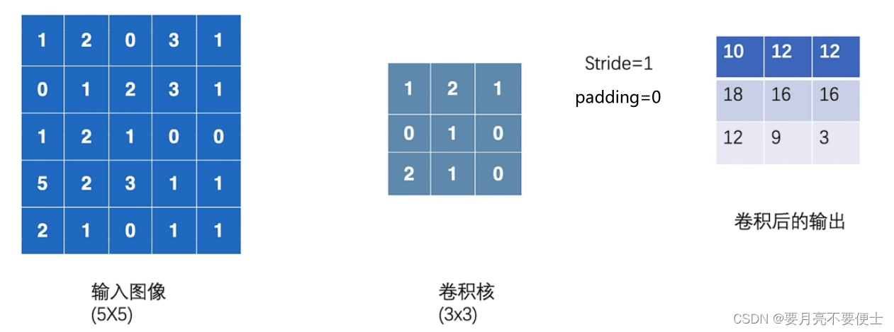
卷积操作
- torch.nn.functional.Conv2d(input, weight, bias, stride, padding)
- 参数input的尺寸要求是(batch_size, channels, h, w)
- 参数weight的尺寸要求是(batch_size, channels, h, w)
- 参数bias是偏置,默认none
- 参数stride是卷积核移动路径,默认为1
- 参数padding是输入两边的填充,默认为0
import torch
import torch.nn.functional as F

# Conv2d(input, weight, bias, stride, padding)
# 参数input的尺寸要求是(batch_size, channels, h, w)
# 参数weight的尺寸要求是(batch_size, channels, h, w)
# 参数bias是偏置,默认none
# 参数stride是卷积核移动路径,默认为1
# 参数padding是输入两边的填充,默认为0

input = torch.tensor([[1, 2, 0, 3, 1],
                      [0, 1, 2, 3, 1],
                      [1, 2, 1, 0, 0],
                      [5, 2, 3, 1, 1],
                      [2, 1, 0, 1, 1]])
kernel = torch.tensor([[1, 2, 1],
                      [0, 1, 0],
                      [2, 1, 0]])
print(input.shape) # torch.Size([5, 5])
print(kernel.shape) # torch.Size([3, 3])

# reshape()参数Tensor为输入
# reshape()参数shape为目标shape,(batch_size, channels, h, w)
input = torch.reshape(input, (1, 1, 5, 5))
kernel = torch.reshape(kernel, (1, 1, 3, 3))
print(input.shape) # torch.Size([1, 1, 5, 5])
print(kernel.shape) # torch.Size([1, 1, 3, 3])

output = F.conv2d(input, kernel, stride=1)
print(output)
# tensor([[[[10, 12, 12],
#           [18, 16, 16],
#           [13,  9,  3]]]])

# 将参数stride改为2(默认为1)
output2 = F.conv2d(input, kernel, stride=2)
print(output2)
# tensor([[[[10, 12],
#           [13,  3]]]])

# 将参数padding改为1(默认为0)
output3 = F.conv2d(input, kernel, padding=1)
print(output3)
# tensor([[[[ 1,  3,  4, 10,  8],
#           [ 5, 10, 12, 12,  6],
#           [ 7, 18, 16, 16,  8],
#           [11, 13,  9,  3,  4],
#           [14, 13,  9,  7,  4]]]])
- 示意图
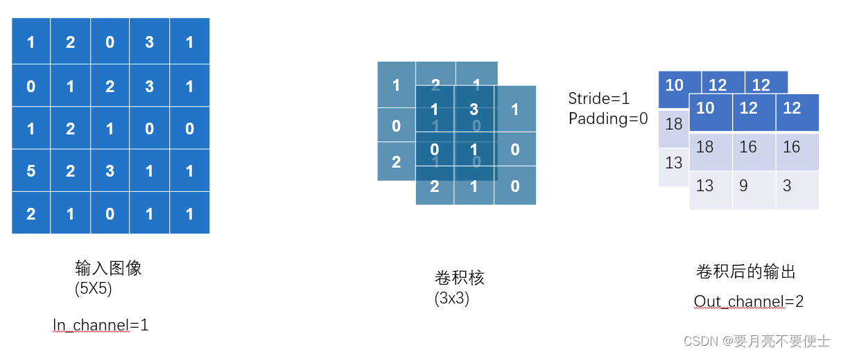
神经网络 - 卷积层
简单介绍
- torch.nn.Conv2d(in_channels, out_channels, kernel_size, stride, padding, padding_mode, dilation, groups, bias)
- in_channels:int,输入图像的通道数
- out_channels:int,输出图像的通道数
- kernel_size:int or tuple,卷积核的尺寸
- stride:int or tuple,卷积核的移动步径,默认1
- padding:int , tuple or str,输入图像周围的填充,默认0
- padding_mode:填充的模式,默认zeros
- dilation:卷积核元素间的距离,默认为1,dilation为1就是卷积核元素间没有距离,这里容易造成误解。
- bias:偏置,为True添加
- 动态观察stride和padding参数的效果
- 注意,我们只需要设定卷积核的尺寸大小,其具体的参数我们不需要去设定,因为神经网络在训练过程中会不断调整卷积核的参数,达到目标。
- 当in_channels=1,卷积核的数目为2时,则out_channels=2,不同层叠加在一块进行输出。
- 我们不需要去考虑卷积核的数目,只需要添加in_channels和out_channels的值。
- 我们不需要去考虑卷积核的数目,只需要添加in_channels和out_channels的值。
- 代码
import torchvision
from torch import nn
from torch.utils.data import DataLoader

dataset = torchvision.datasets.CIFAR10("./dataset", train=False, transform=torchvision.transforms.ToTensor(),
                                       download=True)
dataloader = DataLoader(dataset, batch_size=64)

class MyModule(nn.Module):
    def __init__(self) -> None:
        super().__init__()
        self.conv1 = nn.Conv2d(in_channels=3, out_channels=6, kernel_size=3, stride=1, padding=0)

    def forward(self, x):
        output = self.conv1(x)
        return output

myModule = MyModule()
print(myModule)
# MyModule(
#   (conv1): Conv2d(3, 6, kernel_size=(3, 3), stride=(1, 1))
# )

for data in dataloader:
    # 获取数据包
    imgs, targets = data
    # 输入 -> 输出
    outputs = myModule(imgs)
    print(imgs.shape) # torch.Size([64, 3, 32, 32]) 通道数3
    print(outputs.shape) # torch.Size([64, 6, 30, 30]) 通道数6
添加tensorboard
- 注意将outputs的6通道转为3通道显示,否则报错。
import torch
import torchvision
from torch import nn
from torch.utils.data import DataLoader
from torch.utils.tensorboard import SummaryWriter

dataset = torchvision.datasets.CIFAR10("./dataset", train=False, transform=torchvision.transforms.ToTensor(),
                                       download=True)
dataloader = DataLoader(dataset, batch_size=64)

class MyModule(nn.Module):
    def __init__(self) -> None:
        super().__init__()
        self.conv1 = nn.Conv2d(in_channels=3, out_channels=6, kernel_size=3, stride=1, padding=0)

    def forward(self, x):
        output = self.conv1(x)
        return output

myModule = MyModule()
print(myModule)
# MyModule(
#   (conv1): Conv2d(3, 6, kernel_size=(3, 3), stride=(1, 1))
# )

writer = SummaryWriter("logs")
step = 0
for data in dataloader:
    imgs, targets = data
    outputs = myModule(imgs)
    # print(imgs.shape) # torch.Size([64, 3, 32, 32]) 通道数3
    # print(outputs.shape) # torch.Size([64, 6, 30, 30]) 通道数6
    writer.add_images("input", imgs, step)

    # 需要注意的是:显示彩色图是3通道,但output为6通道,因此需要reshape。[64, 6, 30, 30]  --> [xxx, 3, 30, 30]
    outputs = torch.reshape(outputs, (-1, 3, 30, 30)) # -1代表不确定,需要计算机去计算
    writer.add_images("output", outputs, step)
    step = step + 1

writer.close()
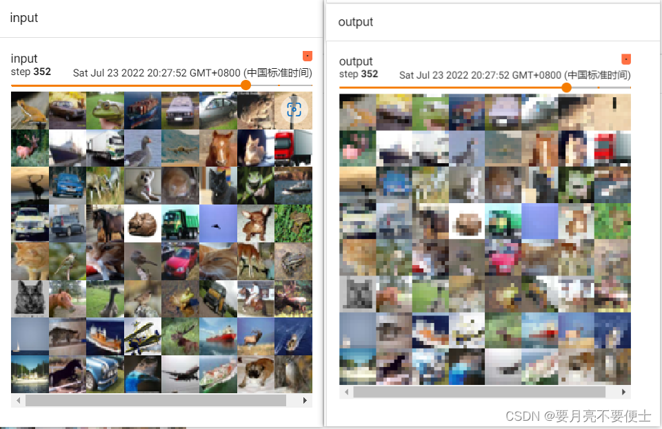
- tensorboard显示

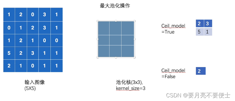
神经网络 - 最大池化层
简单使用
- 最大池化层也称做向下采样层
- torch.nn.MaxPool2d(kernel_size, stride=None, padding=0, dilation=1, return_indices=False, ceil_mode=False)
- kernel_size:卷积核的尺寸,int or tuple
- stride:卷积核的移动步径,默认值就是kernel_size
- padding:输入图像周围的填充
- dilation:卷积核数值间的距离,默认为1,就是没有距离,这里容易造成误解
- ceil_mode:True为ceil模式,保留余下的数据,False为floor模式,丢弃余下的数据
- 最大池化操作演示
- 注意最大池化层要求输入的数据是浮点型,注意数据类型转换。
import torch

# MaxPool2d(kernel_size, stride = kernel_size, padding = 0, dilation = 1, return_indices=False,
# ceil_mode = False)
# 参数kernel_size
# 参数stride默认为kernel_size
# 参数ceil_mode为True时,ceil模式,保留:为False时,floor模式,丢弃。
# 输入shape是(N, C, H, W),输出shape是(N, C, H, W)
from torch import nn
from torch.nn import MaxPool2d

# 池化层要求数据是浮点型
# 否则报错 RuntimeError: "max_pool2d" not implemented for 'Long'
input = torch.tensor([[1, 2, 0, 3, 1],
                      [0, 1, 2, 3, 1],
                      [1, 2, 1, 0, 0],
                      [5, 2, 3, 1, 1],
                      [2, 1, 0, 1, 1]], dtype=torch.float32)
# 输入的shape是(N, C, H, W)
input = torch.reshape(input, (-1, 1, 5, 5))
print(input.shape)

class MyModule(nn.Module):
    def __init__(self) -> None:
        super().__init__()
        self.maxpool1 = MaxPool2d(kernel_size=3, ceil_mode=False)

    def forward(self, x):
        output = self.maxpool1(x)
        return output

myModule = MyModule()
output = myModule(input)
print(output)
# 当ceil_mode为True时,为ceil模式,输出为
# tensor([[[[2., 3.],
#           [5., 1.]]]])
# 当ceil_mode为False时,为floor模式,输出为
# tensor([[[[2.]]]])
作用
- 保留数据特征的同时,减少数据量
import torchvision
from torch import nn
from torch.nn import MaxPool2d
from torch.utils.data import DataLoader
from torch.utils.tensorboard import SummaryWriter

dataset = torchvision.datasets.CIFAR10("./dataset", train=True, transform=torchvision.transforms.ToTensor(),
                                       download=True)
dataloader = DataLoader(dataset, batch_size=64)

class MyModule(nn.Module):
    def __init__(self) -> None:
        super().__init__()
        self.maxpool1 = MaxPool2d(kernel_size=3, ceil_mode=False)

    def forward(self, x):
        output = self.maxpool1(x)
        return output

myModule = MyModule()

writer = SummaryWriter("logs")
step = 0
for data in dataloader:
    imgs, targets = data
    writer.add_images("input", imgs, step)
    outputs = myModule(imgs)
    writer.add_images("output", outputs, step)
    step += 1
writer.close()
- tensorboard显示
神经网络 - 非线性激活
ReLU
- 此版本torch的ReLU层对输入没有shape要求,低版本可能会要求(N, *)尺寸
- 参数inplace,是否在原位置修改
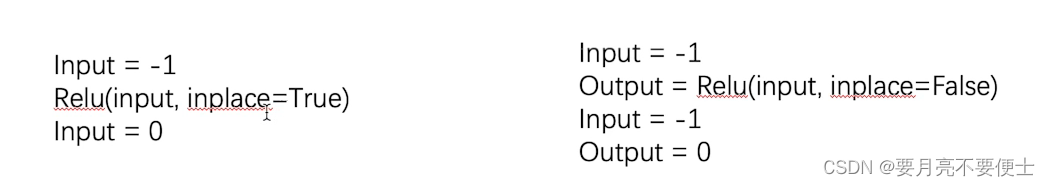
import torch

# ReLU()
# 小于0,截断为0,大于0,y=x
# 参数inplace,是否在原位置修改,若input=-1,经过ReLU(input, inplace=True),则input=0;
# 经过output = ReLU(input, inplace=False),则input仍为-1,output=0
from torch import nn
from torch.nn import ReLU

input = torch.tensor([[1, -0.5],
                      [-1, 3]])

# 此版本torch的ReLU层对输入没有shape要求,低版本可能会要求(N, *)尺寸

class MyModule(nn.Module):
    def __init__(self) -> None:
        super().__init__()
        self.relu1 = ReLU(inplace=False)

    def forward(self, x):
        output = self.relu1(x)
        return output

myModule = MyModule()
output = myModule(input)
print(output)
# tensor([[1., 0.],
#         [0., 3.]])
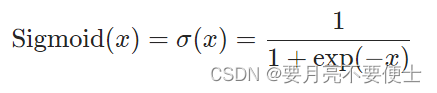
Sigmoid
- 原理
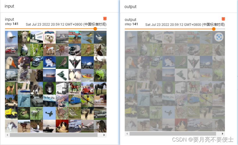
- 代码
import torchvision
from torch import nn
from torch.nn import Sigmoid
from torch.utils.data import DataLoader
from torch.utils.tensorboard import SummaryWriter

dataset = torchvision.datasets.CIFAR10("./dataset", train=False, download=True,
                                       transform=torchvision.transforms.ToTensor())
dataloader = DataLoader(dataset, batch_size=64)

class MyModule(nn.Module):
    def __init__(self) -> None:
        super().__init__()
        self.sigmoid1 = Sigmoid()

    def forward(self, x):
        output = self.sigmoid1(x)
        return output

myModule = MyModule()

writer = SummaryWriter("logs")
step = 0
for data in dataloader:
    imgs, targets = data
    writer.add_images("input", imgs, step)
    outputs = myModule(imgs)
    writer.add_images("output", outputs, step)
    step += 1
writer.close()
- tensorboard显示
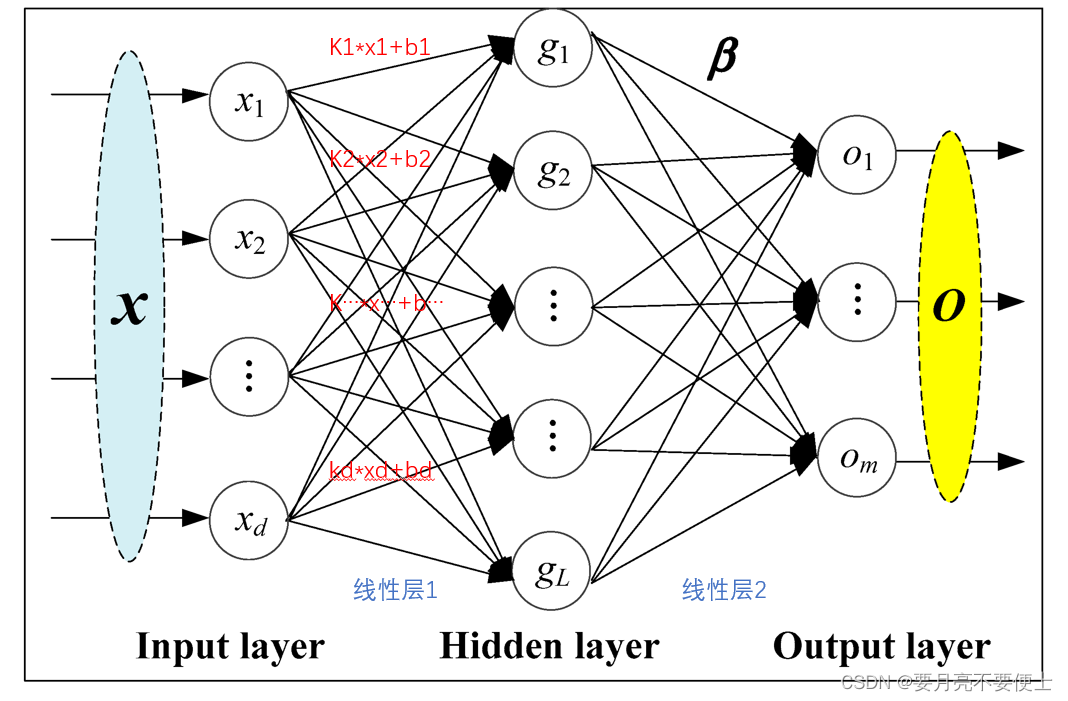
神经网络 - 线性层
简单介绍
-
针对数据特征的变换
-
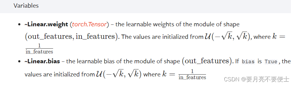
torch.nn.Linear(in_features, out_features, bias=True, device=None, dtype=None)
-
参数in_feartures代表输入层的特征数
-
参数out_features代表输出层的特征数
-
参数bias代表偏置
-
对于上图来说,第一个线性层中,in_features为d,out_features为L。第二个线性层中,in_features为L,out_features为m。
-
线性层中涉及两个变量,weight和bias,即上图中的k和b。
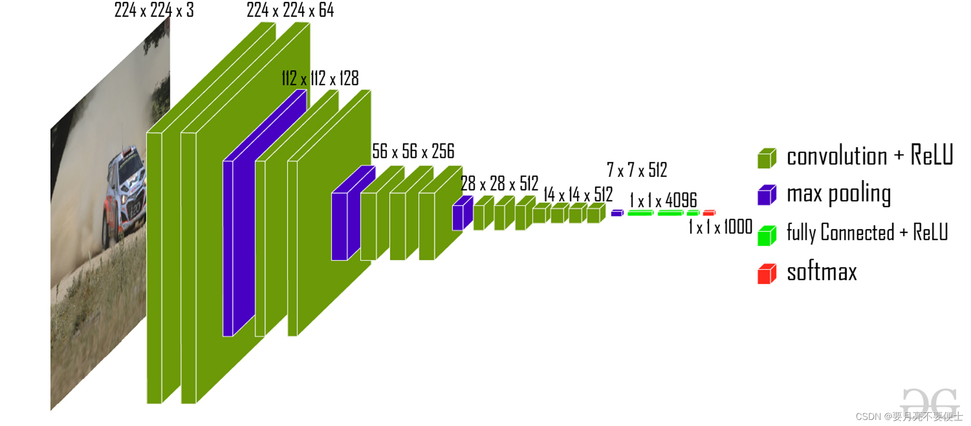
VGG16网络中的线性层实现
简单介绍
- 在经典VGG16网络中,最后1x1x4096到1x1x1000的变化,便是线性层的作用。
# Linear(in_features, out_features)
# 参数in_features为输入层的特征数
# 参数out_features为输出层的特征数
import torch
import torchvision
from torch import nn
from torch.nn import Linear
from torch.utils.data import DataLoader

dataset = torchvision.datasets.CIFAR10("./dataset", train=False, download=True,
                                       transform=torchvision.transforms.ToTensor())

dataloader = DataLoader(dataset, batch_size=64)


class MyModule(nn.Module):
    def __init__(self) -> None:
        super().__init__()
        self.linear1 = Linear(196608, 1000)

    def forward(self, x):
        x = self.linear1(x)
        return x

myModule = MyModule()

for data in dataloader:
    imgs, targets = data
    # print(imgs.shape) # torch.Size([64, 3, 32, 32])
    imgs = torch.reshape(imgs, (1, 1, 1, -1)) # torch.Size([1, 1, 1, 196608])
    outputs = myModule(imgs) # torch.Size([1, 1, 1, 1000])
    # print(outputs.shape)
- 由于涉及将shape由(N, C , H, W)转换成(1, 1, 1, *),改进reshape(),使用
flatten()
...
for data in dataloader:
    imgs, targets = data
    # print(imgs.shape) # torch.Size([64, 3, 32, 32])
    # imgs = torch.reshape(imgs, (1, 1, 1, -1)) # torch.Size([1, 1, 1, 196608])
    imgs = torch.flatten(imgs) # torch.Size([196608])
    outputs = myModule(imgs) # torch.Size([1, 1, 1, 1000])<-reshpae()  # torch.Size([1008])<-flatten()
    # print(outputs.shape)
注意
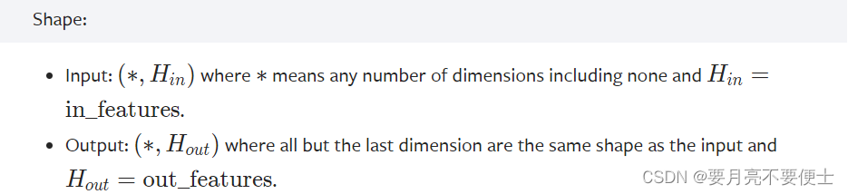
- 虽然举例VGG16网络中的线性层是在一维特征上进行的变换,但不代表线性层的输入shape只能是
(1, 1, 1, *)这种形式。 - 看1.12.0版本的torch官方文档,Linear层多维变换都可以。
搭建网络模型和Sequential使用
CIFAR10网络模型
-
以
CIFAR10 mode为例,建立网络模型,其结构图如下
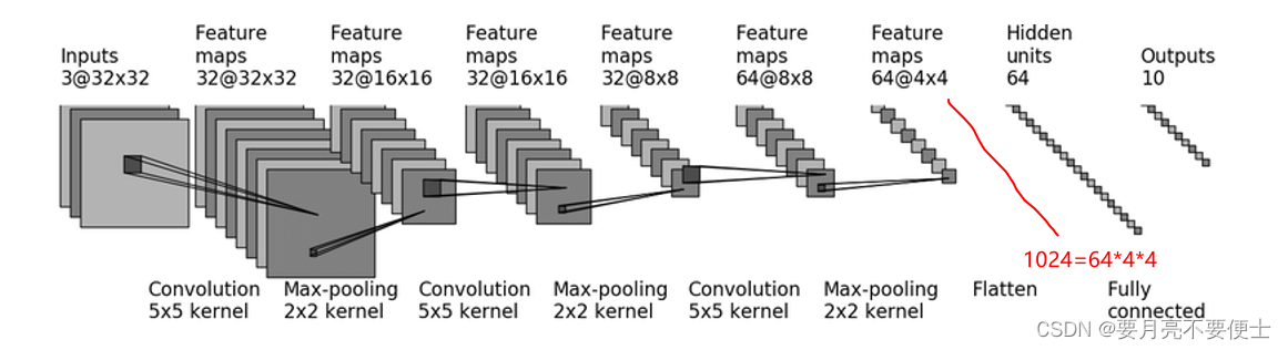
-
再根据神经网络结构图,搭建网络模型时,需要计算的是卷积层中的stride和padding。
-
根据官方提供的计算公式,如下:
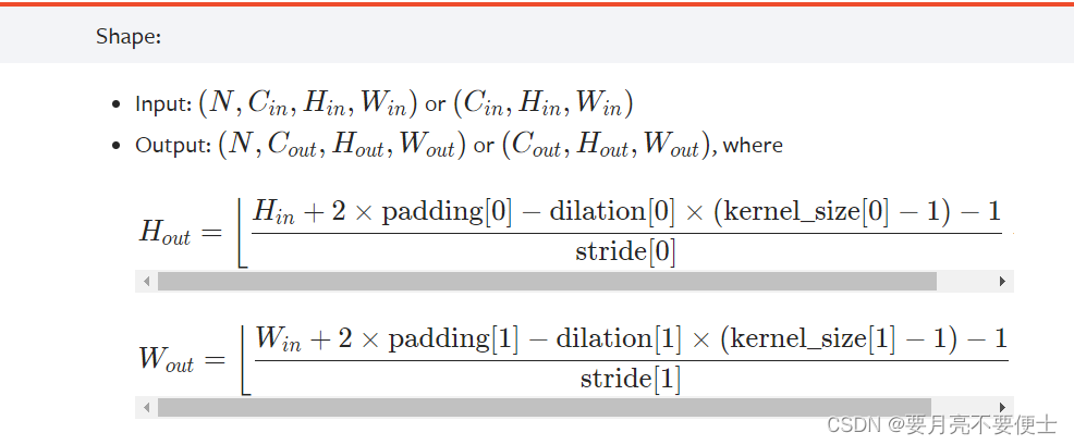
-
以第一层卷积层为例子,
in_channels = 3,out_channels=32; Hin=32,Win=32;Hout=32,Wout=32; kernel_size=5 -
注意,当stride/padding/dilation为int时,其sride[0]=stride[1]=int,padding[0]=padding[1]=int,dilation[0]=dilation[1]=int。
-
将已知量带入公式,可计算得到stride=1,padding=2。
-
搭建网络模型代码
import torch
from torch import nn
from torch.nn import Conv2d, MaxPool2d, Flatten, Linear


class MyModule(nn.Module):
    def __init__(self) -> None:
        super().__init__()
        self.conv1 = Conv2d(3, 32, 5, stride=1, padding=2) # dilation默认为1
        self.maxpool1 = MaxPool2d(2)
        self.conv2 = Conv2d(32, 32, 5, stride=1, padding=2)
        self.maxpool2 = MaxPool2d(2)
        self.conv3 = Conv2d(32, 64, 5, stride=1, padding=2)
        self.maxpool3 = MaxPool2d(2)
        self.flatten = Flatten() # flatten()也有其对应的Flatten层,摊平层
        self.linear1 = Linear(64*4*4, 64)
        self.linear2 = Linear(64, 10)

    def forward(self, x):
        x = self.conv1(x)
        x = self.maxpool1(x)
        x = self.conv2(x)
        x = self.maxpool2(x)
        x = self.conv3(x)
        x = self.maxpool3(x)
        x = self.flatten(x)
        x = self.linear1(x)
        x = self.linear2(x)
        return x

myModule = MyModule()
print(myModule)
# MyModule(
#   (conv1): Conv2d(3, 32, kernel_size=(5, 5), stride=(1, 1), padding=(2, 2))
#   (maxpool1): MaxPool2d(kernel_size=2, stride=2, padding=0, dilation=1, ceil_mode=False)
#   (conv2): Conv2d(32, 32, kernel_size=(5, 5), stride=(1, 1), padding=(2, 2))
#   (maxpool2): MaxPool2d(kernel_size=2, stride=2, padding=0, dilation=1, ceil_mode=False)
#   (conv3): Conv2d(32, 64, kernel_size=(5, 5), stride=(1, 1), padding=(2, 2))
#   (maxpool3): MaxPool2d(kernel_size=2, stride=2, padding=0, dilation=1, ceil_mode=False)
#   (flatten): Flatten(start_dim=1, end_dim=-1)
#   (linear1): Linear(in_features=1024, out_features=64, bias=True)
#   (linear2): Linear(in_features=64, out_features=10, bias=True)
# )

# 测试搭建网络是否正确
input = torch.ones((64, 3, 32, 32)) # batch_size不可缺少,卷积层需要,可简单理解为多少张图片
output = myModule(input)
print(output.shape) # torch.Size([64, 10]) 检验正确
Sequential类
- 利用sequential简化上述代码
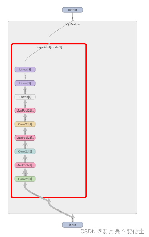
- 添加tensorboard显示网络骨架
import torch
from torch import nn
from torch.nn import Conv2d, MaxPool2d, Flatten, Linear, Sequential


class MyModule(nn.Module):
    def __init__(self) -> None:
        super().__init__()
        self.model1 = Sequential(
            Conv2d(3, 32, 5, stride=1, padding=2),  # dilation默认为1
            MaxPool2d(2),
            Conv2d(32, 32, 5, stride=1, padding=2),
            MaxPool2d(2),
            Conv2d(32, 64, 5, stride=1, padding=2),
            MaxPool2d(2),
            Flatten(),
            Linear(64*4*4, 64),
            Linear(64, 10)
        )

    def forward(self, x):
        x = self.model1(x)
        return x

myModule = MyModule()
print(myModule)
# MyModule(
#   (model1): Sequential(
#     (0): Conv2d(3, 32, kernel_size=(5, 5), stride=(1, 1), padding=(2, 2))
#     (1): MaxPool2d(kernel_size=2, stride=2, padding=0, dilation=1, ceil_mode=False)
#     (2): Conv2d(32, 32, kernel_size=(5, 5), stride=(1, 1), padding=(2, 2))
#     (3): MaxPool2d(kernel_size=2, stride=2, padding=0, dilation=1, ceil_mode=False)
#     (4): Conv2d(32, 64, kernel_size=(5, 5), stride=(1, 1), padding=(2, 2))
#     (5): MaxPool2d(kernel_size=2, stride=2, padding=0, dilation=1, ceil_mode=False)
#     (6): Flatten(start_dim=1, end_dim=-1)
#     (7): Linear(in_features=1024, out_features=64, bias=True)
#     (8): Linear(in_features=64, out_features=10, bias=True)
#   )
# )

# 测试搭建网络是否正确
input = torch.ones((64, 3, 32, 32)) # batch_size不可缺少,卷积层需要,可简单理解为多少张图片
output = myModule(input)
print(output.shape) # torch.Size([64, 10]) 检验正确

# 添加tensorboard显示网络骨架
writer = SummaryWriter("logs")
writer.add_graph(model=myModule, input_to_model=input)
writer.close()
- tensorboard显示 – 双击放大
损失函数和反向传播
- 损失函数的作用
- 计算实际输出和目标之间的差距
- 为我们更新输出提供一定的依据(反向传播)
L1Loss 和 MSELoss
- 此版本torch(1.12.0)对输入和目标shape无要求,均为(*)
- 但input.shape和target.shape要一致
- 输入和目标的数据要为浮点型
# torch.nn.L1Loss(size_average=None, reduce=None, reduction='mean')
# L1Loss类对输入和目标shape无要求,都是(*)
import torch
from torch.nn import L1Loss
from torch import nn

# L1Loss要求输入数据是浮点形
inputs = torch.tensor([1, 2, 3], dtype=torch.float32)
targets = torch.tensor([1, 2, 5], dtype=torch.float32)

loss = L1Loss() # 默认 reduction = “mean"
result = loss(inputs, targets) # tensor(0.6667)
print(result)

# torch.nn.MSELoss(size_average=None, reduce=None, reduction='mean')
# # MSELoss类对输入和目标shape无要求,都是(*)

# 平方差Loss
loss_mse = nn.MSELoss()
result2 = loss_mse(inputs, targets) # tensor(1.3333)
print(result2)

# 交叉熵Loss
input = torch.tensor([0.1, 0.2, 0.3])
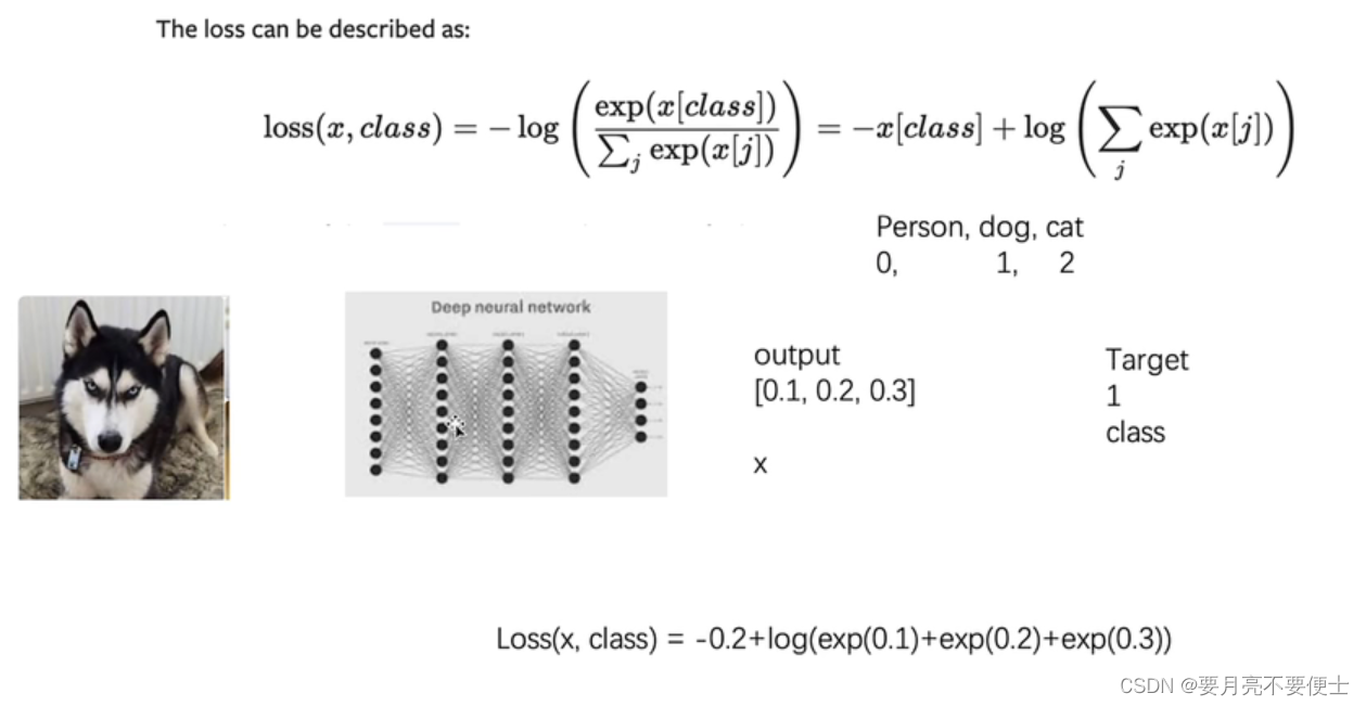
CrossEntropyLoss
- 交叉熵Loss
- 适用于分类问题中
- torch.nn.CrossEntropyLoss(weight=None, size_average=None, ignore_index=- 100, reduce=None, reduction=‘mean’, label_smoothing=0.0)
- 按照输入shape为 (N, C),目标shape为 (N)
- 其中C= number of classes ; N = batch size
- 举例
- 代码
# 交叉熵Loss
# CrossEntropyLoss()
# 按照输入shape为(N, C),目标shape为(N)
# 其中N = number of classes  N = batch size
import torch
from torch import nn

input = torch.tensor([0.1, 0.2, 0.3])
target = torch.tensor([1])
loss_cross = nn.CrossEntropyLoss()
# 输入shape需要为(N, C)
input = torch.reshape(input, (1, 3))
result3 = loss_cross(input, target)
print(result3)
网络中损失函数的计算和反向传播
- 反向传播:计算节点梯度,优化网络中的参数
import torchvision
from torch import nn
from torch.nn import Sequential, Conv2d, MaxPool2d, Flatten, Linear
from torch.utils.data import DataLoader

dataset = torchvision.datasets.CIFAR10("./dataset", train=False, download=True,
                                       transform=torchvision.transforms.ToTensor())
dataloader = DataLoader(dataset, batch_size=1)

class MyModule(nn.Module):
    def __init__(self) -> None:
        super().__init__()
        self.model1 = Sequential(
            Conv2d(in_channels=3, out_channels=32, kernel_size=5, stride=1, padding=2),
            MaxPool2d(kernel_size=2),
            Conv2d(in_channels=32, out_channels=32, kernel_size=5, stride=1, padding=2),
            MaxPool2d(kernel_size=2),
            Conv2d(32, 64, 5, padding=2),
            MaxPool2d(2),
            Flatten(),
            Linear(1024, 64),
            Linear(64, 10),
        )

    def forward(self, x):
        y = self.model1(x)
        return y

myModule = MyModule()
# 交叉熵损失
loss = nn.CrossEntropyLoss()
for data in dataloader:
    imgs, targets = data
    outputs = myModule(imgs)
    # outputs --> tensor([[-0.1541, -0.0937, -0.0411,  0.0405,  0.0265, -0.0111,  0.0820, -0.1124,
    #           0.0817, -0.0898]], grad_fn=<AddmmBackward0>)
    # targets --> tensor([7])
    result_loss = loss(outputs, targets) # result_loss --> tensor(2.2170, grad_fn=<NllLossBackward0>)
    # 反向传播,计算节点梯度,根据梯度来优化网络参数
    result_loss.backward()
优化器
简单使用
- 优化器根据梯度对参数进行调整,降低损失
- *torch.optim.SGD(params, lr=, momentum=0, dampening=0, weight_decay=0, nesterov=False, , maximize=False, foreach=None)
- 参数params代表网络模型中的参数
- 参数lr = learining rate,学习速率。
- lr不能太大,也不能太小,太大会造成模型训练起来不稳定,太小训练比较慢。
- 建议刚开始lr大一些,后面就小一些。
- 其余参数为算法SGD本身特有的,初学时可以直接使用默认即可。
- 使用三步走:
- 对每个节点对应的梯度清0。
optim.zero_grad() - 反向传播,计算节点梯度。
result_loss.backward() - 根据节点中的梯度对参数进行调优。
optim.step()
- 对每个节点对应的梯度清0。
# torch.optim.SGD(params, lr=<required parameter>, momentum=0, dampening=0, weight_decay=0, nesterov=False, *, maximize=False, foreach=None)
# 参数params代表网络模型中的参数
# 参数lr = learining rate,学习速率。
# lr不能太大,也不能太小,太大会造成模型训练起来不稳定,太小训练比较慢。
# 建议刚开始lr大一些,后面就小一些。
# 其余参数为算法SGD本身特有的,初学时可以直接使用默认即可。
import torch
import torchvision
from torch import nn
from torch.nn import Sequential, Conv2d, MaxPool2d, Flatten, Linear
from torch.utils.data import DataLoader

dataset = torchvision.datasets.CIFAR10("./dataset", train=False, download=True,
                                       transform=torchvision.transforms.ToTensor())
dataloader = DataLoader(dataset, batch_size=1)

class MyModule(nn.Module):
    def __init__(self) -> None:
        super().__init__()
        self.model1 = Sequential(
            Conv2d(in_channels=3, out_channels=32, kernel_size=5, stride=1, padding=2),
            MaxPool2d(kernel_size=2),
            Conv2d(in_channels=32, out_channels=32, kernel_size=5, stride=1, padding=2),
            MaxPool2d(kernel_size=2),
            Conv2d(32, 64, 5, padding=2),
            MaxPool2d(2),
            Flatten(),
            Linear(1024, 64),
            Linear(64, 10),
        )

    def forward(self, x):
        y = self.model1(x)
        return y

myModule = MyModule()

# 损失函数
loss = nn.CrossEntropyLoss()
# 优化器
optim = torch.optim.SGD(myModule.parameters(), lr = 0.01)
for data in dataloader:
    imgs, targets = data
    outputs = myModule(imgs)
    result_loss = loss(outputs, targets)
    # 对每个节点对应的梯度清0,由于上一次的梯度对于本次的梯度更新是没有用处的。
    optim.zero_grad()
    # 反向传播,计算节点梯度
    result_loss.backward()
    # 根据节点中的梯度对参数进行调优
    optim.step()
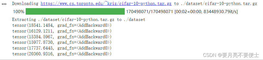
epoch - 多轮训练(类似于多打几轮牌)
- 单纯进行一轮训练,没有任何意义,需要进行多轮训练。
- 损失看的是进行一轮训练损失的总和。
- 注意以下程序的结果,通过google colab跑出,自己电脑上没有英伟达GPU。
import torch
import torchvision
from torch import nn
from torch.nn import Sequential, Conv2d, MaxPool2d, Flatten, Linear
from torch.utils.data import DataLoader

dataset = torchvision.datasets.CIFAR10("./dataset", train=False, download=True,
                                       transform=torchvision.transforms.ToTensor())
dataloader = DataLoader(dataset, batch_size=1)

class MyModule(nn.Module):
    def __init__(self) -> None:
        super().__init__()
        self.model1 = Sequential(
            Conv2d(in_channels=3, out_channels=32, kernel_size=5, stride=1, padding=2),
            MaxPool2d(kernel_size=2),
            Conv2d(in_channels=32, out_channels=32, kernel_size=5, stride=1, padding=2),
            MaxPool2d(kernel_size=2),
            Conv2d(32, 64, 5, padding=2),
            MaxPool2d(2),
            Flatten(),
            Linear(1024, 64),
            Linear(64, 10),
        )

    def forward(self, x):
        y = self.model1(x)
        return y

myModule = MyModule()

# 损失函数
loss = nn.CrossEntropyLoss()
# 优化器
optim = torch.optim.SGD(myModule.parameters(), lr = 0.01)

for epoch in range(20):
    running_loss = 0.0
    for data in dataloader:
        imgs, targets = data
        outputs = myModule(imgs)
        result_loss = loss(outputs, targets)
        # 对每个节点对应的梯度清0,由于上一次的梯度对于本次的梯度更新是没有用处的。
        optim.zero_grad()
        # 反向传播,计算节点梯度
        result_loss.backward()
        # 根据节点中的梯度对参数进行调优
        optim.step()
        running_loss = running_loss + result_loss
    print(running_loss)
- colab结果


 340
340


 被折叠的 条评论
为什么被折叠?
被折叠的 条评论
为什么被折叠?
 到【灌水乐园】发言


